Reading G matrices • hsquared

Teaching panel of an illustrative two-trait genetic covariance matrix G0 beside its genetic-correlation triangle r_g. Mass and length show a positive correlation; values are illustrative. Experimental opt-in multivariate; rotation-invariant; loadings not shown; point display only.

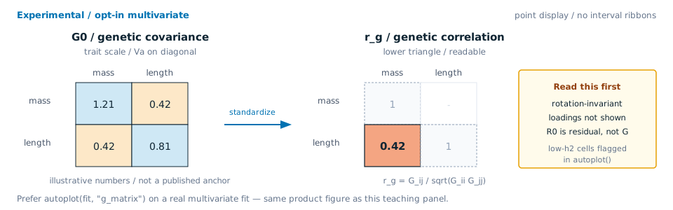
G0 is trait-scale genetic covariance; r_g is the standardized triangle you usually read first. Illustrative numbers — not a published anchor. Prefer autoplot(fit, “g_matrix”) on a real fit (same product figure).

autoplot(fit_mv_plot, "g_matrix")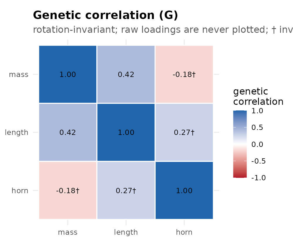

Illustrative data. Experimental / opt-in multivariate genetic-correlation triangle from autoplot(); rotation-invariant; loadings not shown; low-h2 cells flagged imprecise.

This article is for the applied moment after a multivariate animal model has fit: you want to know what the genetic covariance matrix says, what the residual matrix says, and where the current evidence boundary is.

The current hsquared multivariate path fits on the default call — a cbind() Gaussian response with an animal() term needs no engine or target argument — but it remains experimental. It estimates an unstructured additive-genetic covariance matrix G and residual covariance matrix R for Gaussian animal models. It is not yet production multi-trait software, and it does not yet provide standard errors, confidence intervals, selection-response predictions, factor-analytic loadings, or a general phenotypic covariance extractor.

Model scale

For the current two-or-more-trait Gaussian animal model,

$\mathrm{vec}(\mathbf a) \sim \mathrm{MVN}\left(\mathbf 0, \mathbf G \otimes \mathbf A\right), \qquad \mathrm{vec}(\mathbf e) \sim \mathrm{MVN}\left(\mathbf 0, \mathbf R \otimes \mathbf I\right).$

A is the additive relationship matrix from the pedigree. G is the trait-by-trait additive-genetic covariance matrix. R is the trait-by-trait residual covariance matrix. The two matrices are on the scale of the response traits after the fixed effects in the formula.

ped <- data.frame(
  id   = c("s1", "s2", "d1", "d2", "o1", "o2", "o3", "o4"),
  sire = c(NA, NA, NA, NA, "s1", "s1", "s2", "s2"),
  dam  = c(NA, NA, NA, NA, "d1", "d2", "d1", "d2")
)
dat <- data.frame(
  id     = ped$id,
  sex    = c("m", "m", "f", "f", "m", "f", "m", "f"),
  age    = c(4, 5, 4, 5, 1, 1, 1, 1),
  weight = c(72, 75, 65, 68, 31, 33, 35, 30),
  length = c(110, 112, 105, 107, 72, 76, 78, 70)
)

fit_mv <- hsquared(
  cbind(weight, length) ~ sex + age + animal(1 | id, pedigree = ped),
  data = dat,
  family = gaussian(),
  REML = TRUE
)

The G matrix

Use G_matrix() when you want the additive-genetic covariance matrix in the language of quantitative genetics. It is an alias for the more explicit genetic_covariance() extractor.

G_matrix(fit_mv)
genetic_covariance(fit_mv)

Read the diagonal as additive-genetic variance for each trait. Larger diagonal entries mean more additive-genetic variation on that trait’s measurement scale.

Read the off-diagonal as additive-genetic covariance between traits. A positive entry means animals with higher additive-genetic values for one trait tend to have higher additive-genetic values for the other. A negative entry means the additive-genetic values tend to move in opposite directions.

For interpretation across traits with different units, use the genetic correlation:

genetic_correlation(fit_mv)

The genetic correlation is standardized, so it is often easier to read than the raw covariance. It is not a causal statement by itself. A correlation tells you how additive-genetic deviations line up in the fitted model; selection response still needs the relevant selection gradient and a clearly defined prediction target.

The R matrix

Use R_matrix() for the residual covariance matrix. It is an alias for residual_covariance().

R_matrix(fit_mv)
residual_covariance(fit_mv)
residual_correlation(fit_mv)

R collects variation not assigned to the additive animal effect or fixed effects in the current model. It can include measurement noise, microenvironment, unmodelled common environment, unmodelled maternal effects, and other residual sources. Do not read a residual correlation as genetic integration.

Heritability and EBVs

For the current animal-plus-residual multivariate model, per-trait heritability is read from the diagonal pieces of G and R:

$h^2_j = \frac{G_{jj}}{G_{jj} + R_{jj}}.$

Use the extractor rather than calculating by hand:

heritability(fit_mv)

Future models with permanent environment, common environment, maternal effects, or genomic effects will need a model-specific phenotypic denominator. That is why this slice does not add a general P_matrix() extractor yet.

Breeding values are returned by animal and trait:

breeding_values(fit_mv)
EBV(fit_mv)

In an unbalanced response matrix, an animal can be missing one trait and still receive breeding values for all traits. The missing trait borrows information through the fitted genetic covariance and the pedigree relationship.

What to trust first

Trust invariant summaries first:

G_matrix(fit) / genetic_covariance(fit);
R_matrix(fit) / residual_covariance(fit);
genetic_correlation(fit) and residual_correlation(fit);
heritability(fit);
breeding_values(fit);
fit_diagnostics(fit).

The rotation-invariant geometry of G is now surfaced (experimental): the genetic eigenstructure via eigen_G(fit) and g_max(fit), and the Hansen & Houle (2008) evolvability measures evolvability(), variance_along_gradient(), respondability(), conditional_evolvability(), autonomy(), and mean_evolvability(). These are functionals of G itself, not of factor loadings, so they are well defined without a rotation convention.

Factor loadings, specific variance, and latent breeding values stay reserved: loading axes are sign- and rotation-nonunique unless the model has a validated constraint or rotation policy. The agreed cross-lane convention is to bridge only rotation-invariant functionals of G (the eigenbasis + the invariants above), never the raw loadings. Until a loading-rotation policy is validated, hsquared keeps the invariant covariance, correlation, eigenstructure, and evolvability geometry as the stable interpretation layer.

Current evidence boundary

The current multivariate surface is covered at validation scale for t=2 unstructured G0/R0 (experimental label retained). k≥3 and genetic_structure = "diagonal" stay experimental. G-geometry extractors remain descriptive (no standard errors).

Covered in the R lane:

cbind() response grammar;
missing response cells preserved as NA and marshalled to Julia NaN;
G/R covariance and correlation extraction;
G_matrix() and R_matrix() aliases over those same fields;
per-trait heritability and cross-trait EBVs;
the rotation-invariant G geometry: eigen_G(), g_max(), and the Hansen & Houle evolvability measures (live-verified against the engine; experimental, no standard errors);
a shared deterministic R/Julia fixture;
an optional sommer comparator for the diagonal-residual version of the shared fixture.

Still planned:

validated, coverage-calibrated standard errors and confidence intervals for G/R entries, correlations, and heritabilities (experimental, asymptotic SEs are already available via covariance_standard_errors() for an unstructured fit — unstructured-only, not coverage-calibrated);
production sparse multivariate fitting;
cov = diag(), cov = lowrank(K), and cov = fa(K) R grammar;
a general P_matrix() extractor with a model-specific estimand.

Background anchors

The reason G matrices matter is classical quantitative genetics: the additive genetic covariance matrix connects multivariate inheritance, constraint, and response to selection. Useful anchors are Lande and Arnold’s correlated-trait selection framework, Kirkpatrick, Lofsvold and Bulmer’s work on genetic covariance functions for growth trajectories, and Hansen and Houle’s evolvability measures for multivariate characters.

For hsquared, the current package reports the fitted G and R matrices and now the rotation-invariant eigenstructure and Hansen & Houle evolvability geometry (experimental, no standard errors). Selection-response and factor-analytic loading interpretation stay behind explicit validation gates (loadings need a validated rotation policy; nothing here is coverage-calibrated).