Multivariate Gaussian animal models • hsquared

Experimental · validation-scale · dense · REML-only. The experimental label is retained. Intervals are asymptotic and not coverage-calibrated. Whether this cbind() route is covered or partial is on Can I fit and report this?; this banner does not flip it.

Use the multivariate path when the same animals have two or more quantitative traits and the question is about genetic covariance: which traits share additive-genetic variation, what are the genetic correlations, and what are the trait-specific heritabilities?

Two things about this path are true at once, and it is worth separating them before anything else. Reaching it is the default: a cbind() Gaussian response with an animal() term routes to the multivariate REML fitter on an ordinary hsquared() call, with no engine or target argument. A 2026-09-02 maintainer sign-off covers the claim at validation scale for t=2 unstructured G0/R0. At that historical promotion, public_covered_count moved to 6; the current R-public count is 7. The experimental label is retained. k≥3 and genetic_structure = "diagonal" stay experimental. Default routing was reachability; that sign-off is the promotion.

The validation ledger records cold-start recovery, one full-unstructured sommer REML comparator, a published supplied-covariance Mrode anchor, and a MCMCglmm Bayesian agreement probe. Note what the Mrode anchor does and does not do: it is a supplied-covariance BLUP/MME target, so it checks fixed effects and breeding values given known G0 and R0; it is not a textbook check on the estimated covariances themselves, and no such textbook number exists (see “Claim boundary” below). That is still not an ASReml-style production multi-trait claim. Report point estimates within the t=2 unstructured covered scope. The examples are not run when this page is built because they require a local Julia, JuliaCall, and a sibling HSquared.jl checkout.

Model

For two traits measured on animal records, the fitted model is

$\mathrm{vec}(\mathbf a) \sim \mathrm{MVN}\left(\mathbf 0, \mathbf G_0 \otimes \mathbf A\right), \qquad \mathrm{vec}(\mathbf e) \sim \mathrm{MVN}\left(\mathbf 0, \mathbf R_0 \otimes \mathbf I\right).$

Here A is the pedigree additive relationship matrix, G0 is the trait-by-trait additive-genetic covariance matrix, and R0 is the trait-by-trait residual covariance matrix. hsquared sends an NA-preserving response matrix to HSquared.jl; missing response cells are masked by the engine. Missing fixed-effect values are still rejected before fitting.

Current syntax

The current live grammar uses a cbind() response and the ordinary animal-model random intercept. Nothing else is needed:

dat <- data.frame(
  id = c("sire", "dam", "calf1", "calf2"),
  sex = c("m", "f", "f", "m"),
  age = c(4, 4, 1, 1),
  weight = c(72, 65, 31, 35),
  length = c(110, NA, 72, 76)
)

ped <- data.frame(
  id = c("sire", "dam", "calf1", "calf2"),
  sire = c(NA, NA, "sire", "sire"),
  dam = c(NA, NA, "dam", "dam")
)

fit_mv <- hsquared(
  cbind(weight, length) ~ sex + age + animal(1 | id, pedigree = ped),
  data = dat,
  family = gaussian(),
  REML = TRUE
)

The first cbind() fit in a session is slower than the univariate first fit (about 40 s on a few hundred records). Later multivariate calls are faster than that first call but still slower than a univariate animal model. A larger pedigree can take minutes, and the call prints no progress.

Read this as one additive animal effect shared across traits. The trait covariances live in G0; the residual covariances live in R0.

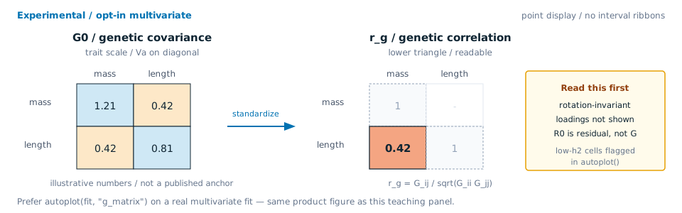
Teaching panel of an illustrative two-trait genetic covariance matrix G0 beside its genetic-correlation triangle r_g. Experimental opt-in multivariate; rotation-invariant; loadings not shown; point display only.

After a multivariate fit, read G0 then the r_g triangle; see Reading G matrices for extractors and autoplot(fit, “g_matrix”).

The explicit spelling still works and still means the same thing, so older scripts do not break:

fit_mv <- hsquared(
  cbind(weight, length) ~ sex + age + animal(1 | id, pedigree = ped),
  data = dat,
  family = gaussian(),
  REML = TRUE,
  control = hs_control(
    engine = "julia",
    engine_control = list(target = "multivariate")
  )
)

engine = "julia" on its own is enough as well: a cbind() response with no target selects the multivariate target. Asking for a univariate target with a cbind() response is still an error rather than a silent reinterpretation.

Like every fitting path in hsquared, this needs the local Julia engine installed; what changed is that you no longer have to name it.

Missing trait cells

Trait cells may be missing in the cbind() response. The dat fixture defined above already shows a valid data shape for the multivariate target: dam’s length is NA, and the fit above still succeeds.

fit_mv <- hsquared(
  cbind(weight, length) ~ sex + age + animal(1 | id, pedigree = ped),
  data = dat,
  family = gaussian(),
  REML = TRUE
)

The missing length value is allowed because it is a response cell. A missing sex, age, or id value would be rejected because those variables define the fixed-effect and random-effect design matrices.

Extracting results

The multivariate fit returns the same kind of object as the univariate fit, plus trait covariance matrices:

genetic_covariance(fit_mv)
residual_covariance(fit_mv)

G_matrix(fit_mv)
R_matrix(fit_mv)

genetic_correlation(fit_mv)
residual_correlation(fit_mv)

heritability(fit_mv)
breeding_values(fit_mv)
fit_diagnostics(fit_mv)

heritability(fit_mv) is per trait. breeding_values(fit_mv) returns EBVs by animal and trait. fit_diagnostics(fit_mv) is the first place to look before interpreting likelihood-based summaries; logLik() and AIC() are intentionally blocked for non-converged multivariate fits.

covariance_standard_errors(fit_mv) returns experimental, asymptotic delta-method standard errors for the G/R covariance and correlation matrices and per-trait h², when a local engine provides them. It mirrors the engine multivariate REML validation row (partial): unstructured-only, REML-only, not coverage-calibrated. The strict per-seed recovery gate is still a non-pass (7/12 seeds), but the 12-seed bias/MCSE study (twin HSquared.jl#78/#79) shows no detectable bias (|bias| ≤ 2·MCSE for all six covariance parameters); reported, not validated.

Initial values

If you supply starting values, use a named list. The names are part of the bridge contract:

fit_mv <- hsquared(
  cbind(weight, length) ~ sex + age + animal(1 | id, pedigree = ped),
  data = dat,
  family = gaussian(),
  REML = TRUE,
  control = hs_control(
    engine_control = list(
      initial = list(
        G0 = diag(1, 2),
        R0 = diag(1, 2)
      )
    )
  )
)

A bare two-element list is rejected because it is too easy to swap genetic and residual covariance starts by accident.

Planned structured grammar

The long-format structured covariance grammar is planned, not implemented:

# Planned, not fitted yet:
y ~ trait + sex + age +
  animal(trait | id, pedigree = ped, cov = us())

# Planned, not fitted yet:
y ~ trait + sex + age +
  animal(trait | id, pedigree = ped, cov = fa(K = 2))

Use the cbind() path above for the current multivariate model. Expert users can select the current rotation-free diagonal-G bridge through engine_control = list(genetic_structure = "diagonal"). That control is still opt-in and experimental. The formula grammar shown here remains reserved for later unstructured, diagonal, low-rank, and factor-analytic covariance models.

Bounded factor-analytic G fit

An explicit expert-control route fits exactly four complete Gaussian traits, one genetic factor, a known pedigree, and trait intercepts. It estimates an unstructured residual covariance. The phenotype data must have a complete four-trait row for every included record.

fit_fa <- hsquared(
  cbind(t1, t2, t3, t4) ~ animal(1 | id, pedigree = ped),
  data = dat,
  family = gaussian(),
  control = hs_control(engine = "julia", engine_control = list(
    target = "multivariate",
    genetic_structure = "factor_analytic",
    rank = 1L,
    julia_project = "/path/to/HSquared.jl",
    iterations = 5000L
  ))
)
G_matrix(fit_fa)
R_matrix(fit_fa)
genetic_correlation(fit_fa)
specific_variance(fit_fa)
fit_diagnostics(fit_fa)

The iterations = 5000L value matches the small live parity fixture; its convergence at the default iteration cap was not established. Inspect fit_diagnostics() on your data. For this FA route it reports the start strategy, number of starts, selected start, objective range, disagreement between fitted covariances, and proximity to the uniqueness floor. Its fa_start_starts entry summarizes validity, convergence, iterations, log-likelihood, minimum uniqueness, and distance from the floor for each attempt. These are optimizer diagnostics, not uncertainty measures. The reported per-trait uniqueness values depend on the fitted loading pattern for separate identification. A fixed rank of one does not guarantee that every uniqueness is identified. This route does not provide structured covariance standard errors or raw-loading inference. It is experimental and partial; the public covered count remains seven. The cov = fa() formula grammar above is still reserved.

What the ordinary-start study found

A frozen 200-seed Gaussian study used 60 pedigree animals, four traits, three complete records per animal, one genetic factor, trait intercepts and an estimated unstructured residual covariance. Each default and balanced start had a 5000-iteration limit. Of all 200 attempts, 141 converged and 110 met the predeclared covariance-recovery diagnostics. There were 59 nonconverged fits, 20 genetic-covariance error classifications and 11 residual-covariance error classifications. The diagnostic recovery fraction was 55%, with a Monte Carlo standard error of 3.52 percentage points and a Wilson 95% interval of 48.1%–61.7%. The study specified no overall pass cutoff.

Near-uniqueness-floor flags occurred in 13 fits, including six classified as recovered; two fits had a better nonconverged start, including one classified as recovered. These flags remain in the counts. Treat returned values from a nonconverged fit as diagnostic output. The covariance thresholds describe this study, and do not establish interval coverage or general optimizer reliability.

Five ordinary-start unit and trait-order checks passed on a separate founder fixture, and one same-model independent R fit agreed with the Julia fit using an informed start. Each result supports its tested fixture and start policy. The fitted covariance still includes both the low-rank part and uniqueness: use the full genetic_covariance(fit_fa) for trait-level genetic summaries.

Claim boundary

This page describes a covered (validation-scale) capability for t=2 unstructured G0/R0 (2026-09-02). The experimental label is retained. k≥3 unstructured fits, diagonal G, and the bounded four-trait FA cell stay experimental/partial. Interval calibration is not claimed.

reached on the default path: a cbind() Gaussian response with an animal() term needs no engine or target argument; the explicit engine = "julia", target = "multivariate" spelling remains accepted;
covered at validation scale for t=2 unstructured; that promotion moved public_covered_count to 6, and the current count is 7. Default routing was reachability; the 2026-09-02 sign-off is the promotion;
Gaussian and REML-only;
animal-model-only;
dense validation-scale;
missing response cells allowed, missing fixed-effect cells rejected;
no cov = us(), cov = diag(), cov = lowrank(K), or cov = fa(K) grammar yet;
R-lane evidence includes a 100-replicate cold-start recovery study, one full-unstructured sommer REML comparator, a published Mrode Example 5.1 supplied-covariance BLUP/MME anchor, and a MCMCglmm Bayesian agreement probe;
no published textbook anchor backs the estimated covariances. Mrode Example 5.1 is a supplied-G0/R0 BLUP/MME anchor: it pins fixed effects and animal BLUPs given known covariances, so it says nothing about whether G0 and R0 are estimated correctly. There is no textbook number for estimated multivariate G0/R0 to check against, so the evidence for the estimated covariances is comparator- and recovery-based (sommer 4.4.5, blupf90+ 2.60, cold-start recovery) rather than textbook-anchored;
R↔︎engine element-wise parity through the bridge has been verified locally at pre-declared tolerances, but not in continuous integration; the CI runner has no Julia, so the parity checks skip there rather than run;
MCMCglmm is Bayesian/MCMC agreement evidence, not same-estimand REML parity.

Use validation_status() and the model-status article for the exact atom table. Report point estimates only within the t=2 unstructured covered scope.