Get Started

Experimental · engine utilities, not a formula API

HSquared.jl is the computational twin of hsquared. Applied users type the R formula. These pages document the engine. Not in Julia General — install with Pkg.add(url = "https://github.com/itchyshin/HSquared.jl"); do not Pkg.add("HSquared") by name. public_covered_count is a claims-register label; read validation_status() rather than a screenshot.

Univariate Gaussian REML (engine utilities). Genomic, QTL, and multivariate routes are separate pages — not this arrow.

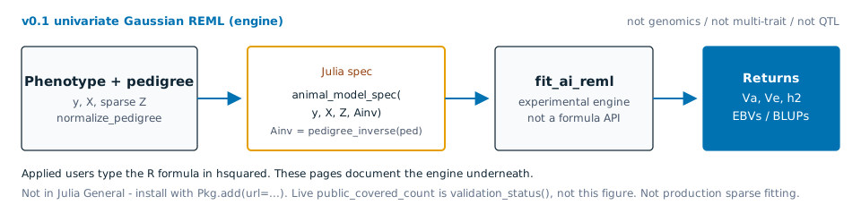
HSquared.jl is the Julia engine twin of hsquared. R users who want a formula should start there. This page walks engine utilities and experimental low-level fitting — not a public formula API.

Route this first

For an applied analysis, start in the hsquared R package. Continue here only when you need an engine utility or want to inspect the Julia layer. Before a fit, use Standard QG models to choose a route and its scope. After a fit, use Validation status before extracting or reporting a point estimate.

Normalize A Pedigree

using HSquared

ped = normalize_pedigree(
    ["offspring", "parent_a", "parent_b"],
    ["parent_a", "0", "0"],
    ["parent_b", "0", "0"],
)

Pedigree(3 animals)

The returned pedigree is sorted so known parents precede offspring.

ped.ids

3-element Vector{String}:
 "parent_a"
 "parent_b"
 "offspring"

Unknown parents are encoded as 0 in the normalized parent-index vectors.

ped.sire, ped.dam

([0, 0, 1], [0, 0, 2])

Build A Sparse Ainv

Ainv = pedigree_inverse(ped)
Matrix(Ainv)

3×3 Matrix{Float64}:
  1.5   0.5  -1.0
  0.5   1.5  -1.0
 -1.0  -1.0   2.0

This matrix is the sparse inverse additive relationship matrix used by later animal-model fitting code.

Validate A Low-Level Model Spec

The first bridge-ready Julia spec validates y, X, Z, Ainv, IDs, family, and ML/REML method. It still does not fit the model.

using LinearAlgebra, SparseArrays

y = [1.0, 2.0, 3.0]
X = [1.0 0.0; 1.0 1.0; 1.0 2.0]
Z = sparse(I, 3, 3)

spec = animal_model_spec(y, X, Z, Ainv; ids = ped.ids, method = "REML")
spec.method

:REML

R bridge code can pass sparse design matrices without densifying by using CSC slots from Matrix::dgCMatrix.

Z_from_slots = sparse_csc_matrix(
    size(Z, 1),
    size(Z, 2),
    Z.colptr .- 1,
    Z.rowval .- 1,
    Z.nzval,
)

Z_from_slots == Z

true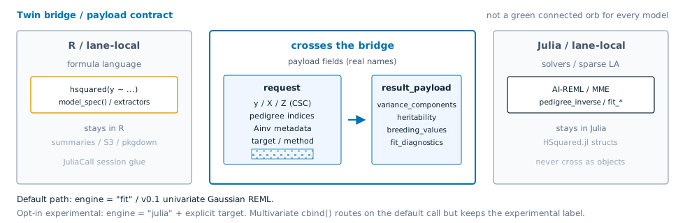

Bridge payload (center) vs lane-local syntax and solvers. Default engine = "fit" is v0.1 only; other models need explicit target. Twin R tour: Fitting models.

The twin R article is Fitting quantitative-genetic models.

Evaluate The Gaussian Likelihood

The first likelihood function evaluates ML or REML at supplied variance components. It is a checked objective value, not an optimizer.

lik = gaussian_loglik(spec, 1.0, 1.0)
lik.loglik

-2.117886169603858

The first sparse likelihood utility evaluates the same REML objective with the Henderson mixed-model-equation determinant identity at supplied variance components.

sparse_lik = sparse_reml_loglik(spec, 1.0, 1.0)
isapprox(sparse_lik.loglik, lik.loglik)

true

Fit Variance Components Experimentally

fit_variance_components optimizes the dense objective for a validated spec. This is the first low-level fitting path, but it is still for tiny validation examples rather than production sparse analysis.

fit = fit_variance_components(spec; initial = (sigma_a2 = 1.0, sigma_e2 = 1.0))
fit.variance_components

(sigma_a2 = 2.140358854918215e-32, sigma_e2 = 5.6043956258172104e-45)

The same dense path is available through the direct bridge-shaped payload:

payload_fit = fit_animal_model(
    y,
    X,
    Z,
    Ainv;
    ids = ped.ids,
    method = :REML,
    initial = (sigma_a2 = 1.0, sigma_e2 = 1.0),
)
payload_fit isa AnimalModelFit

true

The sparse REML validation optimizer uses sparse_reml_loglik() inside the objective. It is REML-only. It is not AI-REML, not the default public R fitting path, and not production sparse fitting.

sparse_fit = fit_sparse_reml(spec; initial = (sigma_a2 = 1.0, sigma_e2 = 1.0))
fit_diagnostics(sparse_fit).target

:sparse_reml

For supplied-variance equation solving, the same validated spec can target Henderson MME explicitly:

target_mme = fit_animal_model(
    spec;
    target = :henderson_mme,
    variance_components = (sigma_a2 = 1.0, sigma_e2 = 1.0),
)
target_mme isa HendersonMMEResult

true

This target is a solver at supplied variance components. It does not estimate variance components and does not return log-likelihood, AIC, df, or optimizer diagnostics.

The dense validation path is size-guarded. The guard is intended for tiny/local bridge checks and fails before the current implementation forms dense covariance or relationship matrices.

try
    fit_variance_components(spec; max_dense_cells = 17)
catch err
    sprint(showerror, err)
end

"ArgumentError: dense validation size nobs^2+nanimals^2 = 18 exceeds max_dense_cells = 17; raise max_dense_cells (engine_control on the R side) or use a sparse route"

Solve Henderson Equations At Supplied Variances

The first sparse equation-solve utility uses Henderson's mixed-model equations at supplied variance components.

mme = henderson_mme(spec, 1.0, 1.0)
fixed_effects(mme)

2-element Vector{Float64}:
 0.9999999999999988
 1.0000000000000009

breeding_values(mme).values

3-element Vector{Float64}:
 4.669885024985544e-16
 1.2264091551091845e-16
 0.0

EBV(mme).values

3-element Vector{Float64}:
 4.669885024985544e-16
 1.2264091551091845e-16
 0.0

This solves for fixed effects and animal-effect BLUPs/EBVs given variance components. It does not estimate those variance components. The same tiny validation path can expose supplied variance components, simple h2, PEV (sparse selected inverse by default for a sparse Ainv), and reliability for the supplied-variance MME result:

variance_components(mme)

(sigma_a2 = 1.0, sigma_e2 = 1.0)

heritability(mme)

0.5

prediction_error_variance(mme).values

3-element Vector{Float64}:
 0.7954545454545452
 0.7954545454545454
 0.9772727272727271

reliability(mme).values

3-element Vector{Float64}:
 0.20454545454545514
 0.20454545454545459
 0.022727272727273373

accuracy(mme) is available only when the derived reliability values are finite and within [0, 1]. It errors instead of clipping validation-scale values outside that range.

The test suite pins the same supplied-variance Henderson fixture as the R twin: sigma_a2 = 1.2, sigma_e2 = 0.8, expected fixed effects, EBVs, fitted values, and h2 = 0.6. That fixture is validation for equation solving only, not variance-component estimation or fitted Mrode output validation.

Extract Experimental Low-Level Results

The dense validation path has first extractors for variance components, fixed effects, breeding values, EBV/BLUP aliases, fitted values, simple univariate heritability, prediction error variance, reliability, and derived accuracy. The variance-component, heritability, PEV, and reliability extractors also accept supplied-variance HendersonMMEResult objects. breeding_values(fit) and fitted_values(fit) use the Henderson MME solve at the fit's variance components.

variance_components(fit)

(sigma_a2 = 2.140358854918215e-32, sigma_e2 = 5.6043956258172104e-45)

breeding_values(fit).values

3-element Vector{Float64}:
 0.0015172475344738042
 0.0007586237672363781
 0.0

BLUP(fit).values

3-element Vector{Float64}:
 0.0015172475344738042
 0.0007586237672363781
 0.0

heritability(fit)

0.9999999999997382

Syntax demonstration, not a heritability estimate

This three-animal toy response is exactly explained by its fixed-effect design. Both fitted variance components are therefore near zero, and the displayed heritability is an unstable ratio of two near-zero numbers. It carries no information about population heritability and must not be interpreted or reported.

prediction_error_variance(fit).values

3-element Vector{Float64}:
 1.1771661456787195e-32
 1.1776201241396396e-32
 2.034640660126846e-32

reliability(fit).values

3-element Vector{Float64}:
 0.45001458845381337
 0.4498024845536299
 0.04939274297319152

accuracy(fit).values

3-element Vector{Float64}:
 0.6704958510379536
 0.670563673584357
 0.22278126563583767

For R bridge work, result_payload returns the current bridge-facing names:

keys(result_payload(fit))

(:variance_components, :heritability, :breeding_values, :fixed_effects, :random_effects, :loglik, :df, :nobs, :predictions, :prediction_error_variance, :reliability, :diagnostics, :converged)

fit_diagnostics() returns compact metadata already stored on the result object:

fit_diagnostics(fit)

(engine = :julia, result_type = :animal_model_fit, target = :variance_components, method = :REML, family = :gaussian, converged = true, optimizer_status = "converged", iterations = 97, loglik = 34.73721724638807, df = 4, nobs = 3, dense_validation_path = true, sparse_mme_path = false, variance_components_source = :estimated_dense_validation)

These outputs are useful for tiny validation examples. They are not yet sparse production EBVs, reliabilities, or prediction error variances.

For fitted AnimalModelFit objects, result_payload(fit) includes prediction_error_variance and reliability as standard (ids, values) fields computed through the :selinv selected-inversion path. The R twin can unpack those top-level fields directly. This is still validation-scale bridge evidence, not a production large-pedigree reliability claim.

For supplied-variance MME results, fit_diagnostics(mme) reports target = :henderson_mme, supplied-variance status, nobs, and loglik = nothing. It does not compute optimizer diagnostics or add log-likelihood output to the Henderson target.

For checking R formula parity before fitting, the R twin also exposes model_spec(). It validates animal(1 | id, pedigree = ped) and previews the bridge payload and Julia targets without executing Julia.

Julia Entry Points and Remaining Gaps

The generic Julia fit_animal_model entry point remains a placeholder. The specialized Julia fitters, including fit_ai_reml, are implemented; the R package dispatches supported models to those fitters through its bridge.

try
    fit_animal_model(nothing)
catch err
    sprint(showerror, err)
end

"fit_animal_model() is not implemented on this route in HSquared.jl. Other model-fitting routes exist; see docs/design/capability-status.md for the current boundary."

Large-pedigree performance hardening, production-scale reliability and prediction-error variance, and relationship-object marshalling beyond sparse Z remain development targets.

R Syntax

R users write the public hsquared syntax. The standard supported route selects the Julia engine automatically; explicit experimental targets use hs_control(engine = "julia"):

hsquared(
  y ~ sex + age + animal(1 | id, pedigree = ped),
  data = dat,
  family = gaussian(),
  control = hs_control(engine = "julia")
)

This R call is executable when the R and Julia packages are installed and the local Julia project is configured. The Julia package supplies the engine pieces; the R package owns formula parsing and the public user interface.

Non-Gaussian marginal caveat

The experimental Poisson and binomial animal-model route defaults to the Laplace marginal approximation. For binary data with one record per latent animal effect, a converged interior Laplace fit can still underestimate the additive latent variance. On the 874-record Plodia pupation full-sib dataset reported in issue #430, Laplace estimated V_A = 0.872, 42% below an exact-likelihood reference (V_A = 1.500); the package's variational fit gave V_A = 1.502 but was substantially slower on that dataset. This is one dataset-specific bias measurement, not a universal correction factor.

For consequential binary analyses, compare marginal = :laplace with marginal = :variational and report the chosen approximation. Their objective values are not directly comparable: the variational value is an evidence lower bound, while the Laplace value approximates the marginal log likelihood.