Multivariate (Multi-Trait) Models

Experimental · validation-scale · dense · REML-only

The experimental label is retained. The R twin exposes cbind() as a public surface — covered-vs-partial is the R limits page, not this engine article. Intervals are not coverage-calibrated. Not ASReml-style production multi-trait software.

G0 is trait-scale genetic covariance; r_g is the standardized triangle. Illustrative numbers. Rotation-invariant — loadings not shown. Twin R article: Reading G matrices.

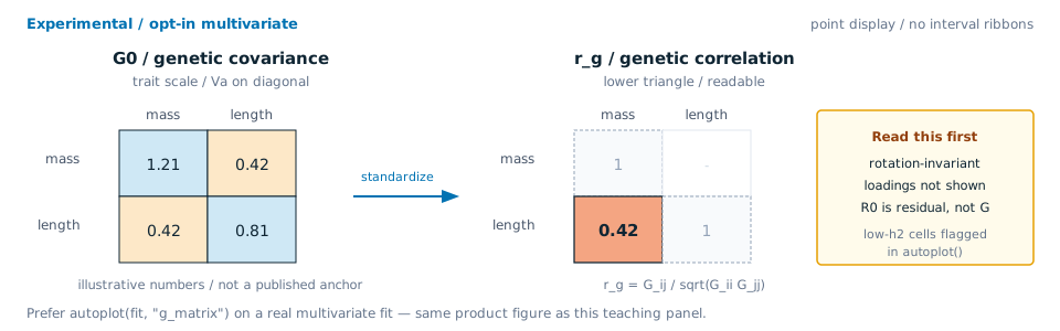
HSquared.jl has a multivariate (multi-trait) animal model engine slice. multivariate_mme solves the balanced multi-trait model at supplied genetic and residual covariance matrices. fit_multivariate_reml estimates those covariances. These are engine APIs. The R twin's cbind() formula is a separate public surface with its own status row — do not read this page as “not wired to R”.

Twin R articles: Multivariate models (cbind() workflow) and Reading G matrices (G₀ / r_g interpretation).

The balanced multi-trait animal model

For t traits, n records, and q related animals:

with phenotype matrix Y (n×t), a fixed-effect design X and a record→animal incidence Z shared across traits, relationship inverse Ainv = A⁻¹ (q×q), additive genetic covariance G0 (t×t), and residual covariance R0 (t×t). Records are ordered individual-major (trait fastest), so the mixed-model equations carry the genetic precision Ainv ⊗ G0⁻¹ on the random block and the residual precision I_n ⊗ R0⁻¹ throughout.

using HSquared, LinearAlgebra

Ainv = pedigree_inverse([1, 2, 3, 4], [0, 0, 1, 1], [0, 0, 2, 2])
Z = Matrix(1.0I, 4, 4)                       # one balanced record per animal
X = ones(4, 1)                               # shared intercept
Y = [10.0 50.0; 12.0 47.0; 9.0 53.0; 11.0 49.0]   # 4 animals × 2 traits
G0 = [1.0 0.4; 0.4 1.5]                      # additive genetic covariance
R0 = [2.0 0.3; 0.3 1.0]                      # residual covariance

fit = multivariate_mme(Y, X, Z, Ainv, G0, R0; traits = ["trait1", "trait2"])
(beta = round.(fit.beta; digits = 4),
 ebv = round.(fit.breeding_values.values; digits = 4))

(beta = [10.4985 49.4054], ebv = [-0.2097 0.9101; 0.2097 -0.9101; -0.0637 1.5558; 0.0696 -0.1775])

The per-trait EBVs are the columns of fit.breeding_values.values (one row per animal). The supplied covariances are echoed back, and the corresponding correlation matrices are derived:

(variance_components = variance_components(fit),
 beta = round.(fixed_effects(fit); digits = 4),
 ebv = round.(EBV(fit).values; digits = 4))

(variance_components = (genetic_covariance = [1.0 0.4; 0.4 1.5], residual_covariance = [2.0 0.3; 0.3 1.0]), beta = [10.4985 49.4054], ebv = [-0.2097 0.9101; 0.2097 -0.9101; -0.0637 1.5558; 0.0696 -0.1775])

(genetic_correlation = round.(fit.genetic_correlation; digits = 4),
 residual_correlation = round.(fit.residual_correlation; digits = 4))

(genetic_correlation = [1.0 0.3266; 0.3266 1.0], residual_correlation = [1.0 0.2121; 0.2121 1.0])

genetic_correlation also works directly on any covariance matrix:

round.(genetic_correlation(G0); digits = 4)

2×2 Matrix{Float64}:
 1.0     0.3266
 0.3266  1.0

Unbalanced / missing-trait records

Most multi-trait analyses are unbalanced — some animals are not measured on every trait. Mark an unobserved trait with missing or NaN in Y. That observation is dropped, and the animal's residual precision uses only its observed-trait submatrix inv(R0[Sᵢ, Sᵢ]). Breeding values are still returned for every animal and trait (the missing traits borrow information through G0):

Ymiss = [10.0 50.0; 12.0 NaN; NaN 53.0; 11.0 49.0]   # animal 2 missing trait2, animal 3 missing trait1
fitm = multivariate_mme(Ymiss, X, Z, Ainv, G0, R0)
round.(fitm.breeding_values.values; digits = 4)

4×2 Matrix{Float64}:
 -0.3567  -0.3305
  0.3567   0.3305
  0.2604   0.9766
 -0.1374  -0.7396

With every trait observed this reduces exactly to the balanced solve above.

Estimating the covariances (REML)

fit_multivariate_reml estimates G0 and R0 by dense REML — maximizing -½(log|V| + log|X'V⁻¹X| + (y−Xβ̂)'V⁻¹(y−Xβ̂)) over a log-Cholesky parameterization that keeps both matrices positive definite. It accepts the same inputs (balanced or with missing records) and returns the estimated covariances, their correlations, per-trait heritabilities, and the breeding values at the estimate:

fitr = fit_multivariate_reml(Y, X, Z, Ainv)
(covariances = variance_components(fitr),
 heritability = round.(heritability(fitr); digits = 3),
 ebv = round.(breeding_values(fitr).values; digits = 3),
 converged = fitr.converged)

(covariances = (genetic_covariance = [1.2365422957655137 -1.9942071489208073; -1.9942071489208073 3.216114941175481], residual_covariance = [0.6182311881180035 -1.4758856047290196; -1.4758856047290196 3.5233396393362337]), heritability = [0.667, 0.477], ebv = [-1.146 1.847; 1.146 -1.847; -0.354 0.572; 0.646 -1.041], converged = true)

The multivariate accessors return copies of matrix and vector fields. They are Julia-side convenience wrappers over the existing result metadata: variance_components, fixed_effects, breeding_values, EBV, BLUP, and heritability for REML results. They do not widen result_payload() or change the R bridge contract.

Experimental estimator · not coverage-calibrated

Multivariate REML is experimental and dense. Engine evidence includes fixture self-consistency plus same-estimand sommer and blupf90+ legs recorded on the V4-MV-REML row — that is not ASReml-style production software, not interval calibration, and not a k≥3 or diagonal-G claim. On small fixtures the optimum can sit on a boundary (a genetic correlation of ±1, or a zero variance).

Structured genetic covariance

Phase 4B adds engine utilities for constrained additive genetic covariance matrices:

The direct matrix builders are diagonal_covariance, lowrank_covariance, and factor_analytic_covariance:

Λ = reshape([0.8, -0.4], 2, 1)
(diag = diagonal_covariance([1.0, 1.5]),
 lowrank = round.(lowrank_covariance(Λ); digits = 3),
 fa = round.(factor_analytic_covariance(Λ, [0.2, 0.3]); digits = 3))

(diag = [1.0 0.0; 0.0 1.5], lowrank = [0.64 -0.32; -0.32 0.16], fa = [0.84 -0.32; -0.32 0.46])

The same structures can constrain the genetic covariance in the dense REML estimator while leaving the residual covariance unstructured. The existing two-trait, one-factor example below is saturated: its fitted Ψ is only one optimizer-selected decomposition of G and must not be interpreted as an identified estimate. The bounded four-trait R route has its own local- identification and fitted-information limits; see the FA design note.

fad = fit_multivariate_reml(
    Y, X, Z, Ainv;
    genetic_structure = :factor_analytic,
    rank = 1,
    initial = (loadings = Λ, uniqueness = [0.2, 0.3], R0 = R0),
)
(G0 = round.(fad.genetic_covariance; digits = 3),
 structure = genetic_structure(fad),
 loadings = round.(genetic_loadings(fad); digits = 3),
 uniqueness_decomposition_diagnostic_only = round.(genetic_uniqueness(fad); digits = 3),
 converged = fad.converged)

(G0 = [1.236 -1.994; -1.994 3.217], structure = (structure = :factor_analytic, rank = 1), loadings = [-1.112; 1.793;;], uniqueness_decomposition_diagnostic_only = [0.0, 0.0], converged = true)

The loadings and uniqueness above expose the fitted decomposition for engine diagnostics; they do not make the decomposition identified. genetic_rank is the requested factor count, traits follow the input Y column order, and mean_evolvability depends on the trait coordinates and units. Directional metrics and genetic PCA axes are also coordinate- and unit-dependent: they use Euclidean unit directions or eigenvectors in the supplied trait scale. The rotation invariance here means invariance to orthogonal latent-factor rotations that preserve G; it does not imply invariance to rescaling traits. Choose and report a scientifically meaningful common scale before comparing directions across traits. The per-trait heritability uses Gᵢᵢ/(Gᵢᵢ + Rᵢᵢ) on the relationship matrix reference scale.

The structured metadata accessors copy existing Julia result fields. They do not change result_payload() or the R bridge contract.

The structured covariance path is experimental and dense/validation-scale. It has deterministic self-consistency tests and an opt-in seeded recovery harness:

julia --project=. sim/phase4_multivariate_reml_recovery.jl
julia --project=. sim/phase4_multivariate_reml_recovery.jl --seeds=20260616
julia --project=. sim/phase4b_structured_covariance_recovery.jl
julia --project=. sim/phase4b_structured_covariance_recovery.jl --case=factor_analytic --seeds=20260614

On an interactive workstation, use a throttled command form for long recovery runs:

env JULIA_NUM_THREADS=1 OPENBLAS_NUM_THREADS=1 OMP_NUM_THREADS=1 VECLIB_MAXIMUM_THREADS=1 nice -n 15 julia --project=. sim/phase4_multivariate_reml_recovery.jl --seeds=20260616

The harnesses are not part of CI. The unstructured harness records two-trait known-truth recovery on a repeated-record half-sib design and accepts --seed or explicit --seeds lists with summaries; the structured harness records low-rank and factor-analytic recovery on a similar design and can run explicit seed lists with per-case summaries. Both use loose, version-robust thresholds. The shared calibration protocol in docs/dev-log/decisions/2026-06-14-multivariate-recovery-calibration-protocol.md defines the seed-count, run-plan, and reporting gate required before any broad multi-seed calibration claim. Phase 4B calibration (2026-06-14; did not pass) was executed on the predeclared seed sets and did not pass: unstructured passed 6/10, factor-analytic passed 8/10, and low-rank passed 9/10, with all fits converged. That Phase 4B 8/10 is not the later S4 covered gate (docs/dev-log/recovery-checkpoints/2026-09-03-v08-s4-fa-d4-k1.md). The raw logs and summary live in docs/dev-log/recovery-checkpoints/. The deterministic helper sim/summarize_recovery_calibration.jl can regenerate the Markdown case summary, failure-mode table, and failed-seed list from those raw logs without rerunning any simulations. The current failure-mode triage is: unstructured has 3 G-only failures plus 1 G+R failure, factor-analytic has 1 G-only failure plus 1 G+R failure, and low-rank has 1 R-only failure. The follow-up decision note docs/dev-log/decisions/2026-06-14-calibration-failure-response.md records that failed seeds cannot be dropped and thresholds cannot be relaxed after seeing the results. The structured path returns sign-canonicalized loading columns: within each factor, the largest-absolute loading is non-negative. This removes arbitrary sign flips from metadata but does not identify rotations or make loading columns uniquely interpretable. The optimizer still searches the full raw loading vector. It does not drop the K(K-1)/2 rotational degrees of freedom of Λ for rank = K >= 2. _mv_nparams subtracts those directions for likelihood-ratio reporting only. converged is still a Nelder-Mead simplex-spread test on the unreduced parameter vector. The current policy is recorded in docs/dev-log/decisions/2026-06-14-loading-rotation-identifiability.md. A passing or revised calibration protocol, covariance standard errors, external-comparator parity, and R-facing multivariate / covariance-structure syntax are still missing.

Multivariate repeatability (animal + permanent environment)

fit_multivariate_repeatability_reml is the experimental dense REML path for repeated-measures multivariate data with additive genetics and an iid permanent-environment term (hsquared #237):

A \neq I separates G_0 from P_0; repeated records separate P_0 from R_0. Animal-only multivariate REML absorbs V_{PE} into G_0. Per-trait heritability uses the PE denominator h^2_k = G_{0,kk}/(G_{0,kk}+P_{0,kk}+R_{0,kk}). This is engine-internal and experimental. No covered flip. The R twin still fences cbind() + permanent() until it lifts the spec gate. The bridge payload is multivariate_repeatability_result_payload (target = "multivariate_repeatability_reml", status = "experimental").

Validation boundary

Covered now (self-consistent, comparator-free):

• multivariate_mme β and EBVs match an independent loop-built multivariate MME and an independent marginal-GLS BLUP;

• it reduces to the univariate animal model when t = 1;

• with diagonal G0, R0 it decouples into t independent single-trait fits;

• unbalanced / missing-trait records are validated the same way (loop-built MME + marginal-GLS with per-individual residual blocks), and reduce to the balanced solve when nothing is missing;

• fit_multivariate_reml is validated by the t = 1 reduction (recovers the univariate REML estimate), the REML log-likelihood matching the univariate package scale, the optimum beating a coarse grid, and EBV consistency with the MME at the estimate;

• opt-in sim/phase4_multivariate_reml_recovery.jl records seeded two-trait known-truth recovery outside CI (G relative error 0.174500, R relative error 0.131056, thresholds 0.25 / 0.20);

• a shared deterministic two-trait CSV fixture in test/fixtures/phase4_multitrait_parity/ records a Julia REML target for R-lane comparator work; its README and docs/dev-log/decisions/2026-06-14-multitrait-comparator-protocol.md define the comparator protocol; CI checks fast self-consistency at the stored target covariances (beta, EBVs, h², and REML log-likelihood), but does not re-run the optimizer or claim external comparator parity;

• structured genetic covariance builders and REML constraints are validated by deterministic constructor identities, metadata checks, returned-loglik equality to the existing evaluator, PSD/PD covariance checks, and constrained fits not exceeding the unstructured REML loglik.

The balanced checks hold to a committed 1e-10 tolerance and the missing-data checks to 1e-9 (the observed agreement is machine precision).

Still planned / coordinated:

• a long-format interface for the missing-record case;

• per-trait fixed-effect and incidence designs;

• multi-seed recovery calibration, covariance standard errors, loading rotation/identifiability conventions, and external-comparator parity (sommer / ASReml / JWAS) for the REML and structured-covariance estimators;

• a published Mrode multi-trait fixture;

• the public R multivariate model-spec mapping — R lane.