Getting started with freqTLS • freqTLS

freqTLS fits single-stage four-parameter logistic (4PL) thermal-load-sensitivity (TLS) / thermal death-time models by maximum likelihood, parameterised directly in CTmax (the critical thermal maximum at the reference time tref) and z (thermal sensitivity, degrees Celsius per order-of-magnitude change in exposure duration). It returns prior-free frequentist confidence intervals — Wald, profile-likelihood (asymmetry-respecting, the default), and bootstrap. It is the likelihood complement to the Bayesian bayesTLS package. The thermal-load-sensitivity modelling framework was introduced by Daniel W. A. Noble, Pieter A. Arnold, and Patrice Pottier; see vignette("comparing-to-bayesTLS") for the comparison boundary.

This vignette walks through the core loop: simulate → fit → confidence intervals → plot. It runs end to end with a small simulation and needs no Stan, no MCMC, and no internet.

library(freqTLS)

Simulate a dataset

simulate_tls() draws survival counts from the locked data-generating process: a factorial grid of assay temperatures and exposure durations, with the 4PL evaluated at the supplied true CTmax, z, and shape parameters. We use the overdispersed beta-binomial family here; phi is its precision parameter — larger phi means less overdispersion, approaching the ordinary binomial as phi grows.

set.seed(1)
dat <- simulate_tls(
  temps  = seq(30, 42, by = 2),
  times  = c(0.5, 1, 2, 4, 8),
  reps   = 3,
  n      = 20,
  CTmax  = 36,
  z      = 4,
  phi    = 50,
  family = "beta_binomial",
  seed   = 1
)
head(dat)
#>   temp duration total survived          p
#> 1   30      0.5    20       20 0.97988215
#> 2   32      0.5    20       18 0.97856626
#> 3   34      0.5    20       20 0.96282035
#> 4   36      0.5    20       17 0.80560767
#> 5   38      0.5    20        3 0.27915697
#> 6   40      0.5    20        2 0.04828075

Each row is one temperature-by-duration cell: survived out of total individuals survived the exposure. The true parameters used to generate the data are kept as an attribute, which is handy for checking recovery:

attr(dat, "truth")[c("CTmax", "z", "phi")]
#> $CTmax
#> [1] 36
#> 
#> $z
#> [1] 4
#> 
#> $phi
#> [1] 50

Standardise and fit the model

freqTLS mirrors the bayesTLS workflow. First standardize_data() names the temperature, duration, and survival-count columns and records the data contract; then fit_4pl() fits the 4PL by maximum likelihood and returns a freq_tls workflow object. t_ref is the reference time at which CTmax is defined, in the same unit as duration; it does not convert the observed durations. When omitted, fit_4pl() and fit_tls() resolve it to one physical hour from a recognised duration_unit (for example, 60 minutes or 1 hour). Bare data without metadata retain the historical one-native-unit fallback with a warning, so use an explicit reference if their unit is not recorded. A supplied numeric reference is never converted: for minute data, t_ref = 1 deliberately means CTmax at one minute, whereas the omitted default is one hour (t_ref = 60).

std <- standardize_data(
  dat,
  temp     = "temp",
  duration = "duration",
  n_total  = "total",
  n_surv   = "survived",
  duration_unit = "hours"
)

fit <- fit_4pl(std, family = "beta_binomial")
fit
#> <freq_tls>
#>   Data:    105 rows; 7 temperatures; 5 durations
#>   T_bar:   36.00
#>   Family:  beta_binomial (relative threshold, t_ref = 1 hours)
#>   Fit:     converged (pdHess = TRUE); default CI method = profile

Formula interface

For the supported moderators, fit_4pl() takes a similar direct interface to bayesTLS — ctmax =, z =, or the by = shorthand (for example, by = "population"). The engine also exposes the explicit 4PL formula grammar through tls_bf(): the response is survival counts, time() identifies duration, and temp() identifies assay temperature. The following formula still fits the single-stage 4PL, not an ordinary linear model; it matches the preceding fit:

fit_f <- fit_tls(
  tls_bf(survived | trials(total) ~ time(duration) + temp(temp)),
  data   = dat,
  family = "beta_binomial",
  tref   = 1
)
all.equal(coef(fit_f), coef(fit))
#> [1] TRUE

The grammar scales well beyond a single ungrouped fit: each sub-parameter can take a grouping factor, a continuous covariate, or an lme4-style random intercept. See Going further below.

The print method reports the headline quantities (CTmax, z), the shape parameters (low, up, k), the overdispersion phi, and the convergence status. summary() adds standard errors and the log-likelihood:

summary(fit)
#> <freqTLS beta_binomial 4PL fit> summary
#> Call: fit_tls(x = ff, family = fam_name, tref = t_ref, start = start, control =
#> control, trace = trace, quiet = quiet, data = data)
#> Reference time (tref): 1 | family: beta_binomial
#> Data: 105 observations, ungrouped
#> 
#> Coefficients (natural scale; Wald z-test):
#>  parameter group estimate std.error z value  Pr(>|z|)
#>        low         0.0328  0.008901   3.685 2.284e-04
#>         up         0.9761  0.009545 102.300 0.000e+00
#>          k         5.4080  0.684200   7.904 2.696e-15
#>      CTmax   all  36.0000  0.129300 278.500 0.000e+00
#>          z   all   3.9010  0.236600  16.490 4.262e-61
#>        phi        26.6800 10.640000   2.507 1.219e-02
#> Optimiser: nlminb | code 0 | pdHess TRUE | converged (pdHess)
#> logLik -152.8 | df 6 | AIC 317.6

A tidy, broom-style table first shows all natural-scale 4PL parameters. Dedicated extractors are useful when a later analysis needs only the headline quantities:

tidy_parameters(fit)
#> # A tibble: 6 × 8
#>   parameter group estimate std.error conf.low conf.high interval_type scale   
#>   <chr>     <chr>    <dbl>     <dbl>    <dbl>     <dbl> <chr>         <chr>   
#> 1 low       NA      0.0328   0.00890   0.0191    0.0557 wald          logit   
#> 2 up        NA      0.976    0.00954   0.957     0.995  wald          identity
#> 3 k         NA      5.41     0.684     4.21      6.95   wald          log     
#> 4 CTmax     all    36.0      0.129    35.7      36.3    wald          identity
#> 5 z         all     3.90     0.237     3.46      4.40   wald          log     
#> 6 phi       NA     26.7     10.6      12.1      58.9    wald          log
get_ctmax(fit)
#> # A tibble: 1 × 8
#>   parameter group estimate std.error conf.low conf.high interval_type scale   
#>   <chr>     <chr>    <dbl>     <dbl>    <dbl>     <dbl> <chr>         <chr>   
#> 1 CTmax     all       36.0     0.129     35.7      36.3 wald          identity
get_z(fit)
#> # A tibble: 1 × 8
#>   parameter group estimate std.error conf.low conf.high interval_type scale
#>   <chr>     <chr>    <dbl>     <dbl>    <dbl>     <dbl> <chr>         <chr>
#> 1 z         all       3.90     0.237     3.46      4.40 wald          log

Profile-likelihood confidence intervals

The reason for the direct CTmax/z parameterisation is that both headline quantities are model parameters, so they can be profiled directly. confint() with method = "profile" (the default) inverts the likelihood-ratio test: the interval is the set of values whose deviance from the maximum stays below the profile- $t$ cutoff (a squared Student- $t$ quantile on the residual degrees of freedom, not $\chi^2_1$ ; see vignette("frequentist-and-bayesian")), found by root-finding on each side of the MLE.

confint(fit, parm = "CTmax", method = "profile")
#> # A tibble: 1 × 8
#>   parameter conf.low conf.high estimate level method  scale    conf.status
#>   <chr>        <dbl>     <dbl>    <dbl> <dbl> <chr>   <chr>    <chr>      
#> 1 CTmax         35.7      36.3     36.0  0.95 profile identity ok
confint(fit, parm = "z", method = "profile")
#> # A tibble: 1 × 8
#>   parameter conf.low conf.high estimate level method  scale conf.status
#>   <chr>        <dbl>     <dbl>    <dbl> <dbl> <chr>   <chr> <chr>      
#> 1 z             3.43      4.38     3.90  0.95 profile log   ok

These are confidence intervals, not posteriors: they carry no prior, and they need not be symmetric about the estimate. The conf.status column reports "ok" when the profile closes on both sides; a weakly identified parameter is flagged rather than given a fabricated bound (see vignette("profile-likelihood")).

For comparison, the first-order Wald interval is available with method = "wald":

confint(fit, parm = c("CTmax", "z"), method = "wald")
#> # A tibble: 2 × 8
#>   parameter conf.low conf.high estimate level method scale    conf.status
#>   <chr>        <dbl>     <dbl>    <dbl> <dbl> <chr>  <chr>    <chr>      
#> 1 CTmax        35.7      36.3     36.0   0.95 wald   identity ok         
#> 2 z             3.46      4.40     3.90  0.95 wald   log      ok

Plot the fit

plot_survival_curves() draws the fitted survival probability against exposure duration, one curve per temperature, with the observed proportions overlaid:

plot_survival_curves(fit)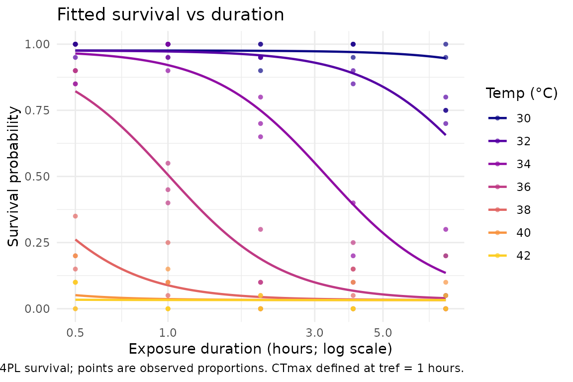

Fitted 4PL survival curves: survival probability declining with exposure duration, one curve per assay temperature, with observed proportions as points.

The default uncertainty display is the Confidence Eye: a pale confidence lens with a hollow point estimate. It is freqTLS’s visual identity and deliberately avoids posterior-density iconography, because these are likelihood intervals. Read the lens width as the confidence interval and the hollow circle as the maximum-likelihood estimate. Do not use overlap as a hypothesis test; inspect the reported contrast or confidence interval for that question. A hollow point with no lens flags a profile that did not close (a weakly identified parameter).

plot_confidence_eye(fit, parm = c("CTmax", "z"), method = "profile")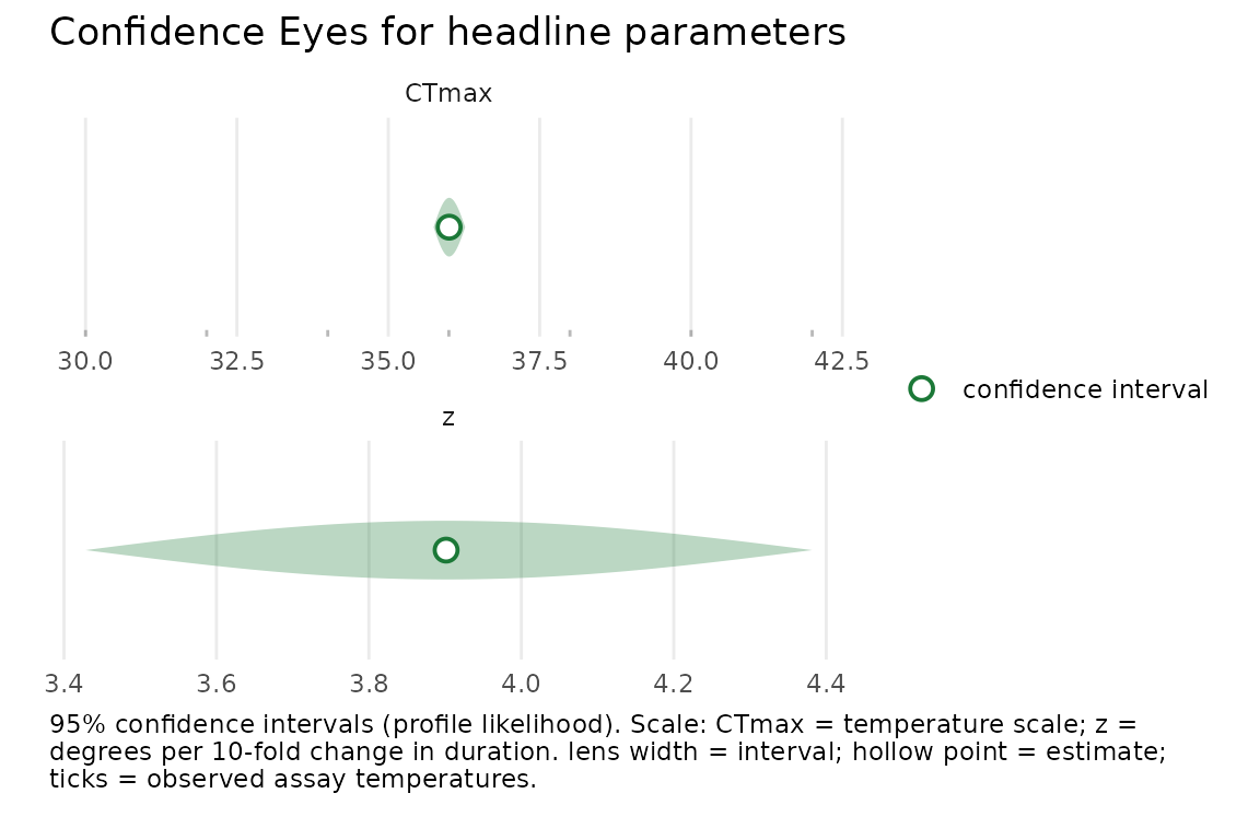

Confidence Eye plot: a pale lens spanning the profile-likelihood interval with a hollow point estimate, for CTmax and z.

Going further: groups, shape predictors, and random effects

The same tls_bf() grammar scales from the single fit above to grouped, covariate, and hierarchical models.

Other families. Besides "beta_binomial", fit_tls() accepts "binomial" (no overdispersion) and "beta" (a continuous proportion in (0, 1) with no trials column; the runnable example below uses simulated beta data).

Grouped CTmax and z. Put a grouping factor on a sub-parameter to estimate a separate, directly profile-able CTmax and z per group, with one shared curve shape (the bayesTLS constant-shape configuration). In the formula, z enters on its internal log scale as log_z (and steepness as log_k), so the grouped term is written log_z ~ group. Intervals are still requested by the natural-scale name (z:cool, not log_z:cool) — confint() converts internally:

dat_grp <- simulate_tls(
  temps = seq(30, 42, by = 2), times = c(0.5, 1, 2, 4, 8), reps = 3, n = 20,
  group = c("cool", "warm"), CTmax = c(34, 38), z = c(3, 5),
  phi = 50, family = "beta_binomial", seed = 2
)
fit_grp <- fit_tls(
  tls_bf(
    survived | trials(total) ~ time(duration) + temp(temp),
    CTmax ~ group,
    log_z ~ group
  ),
  data = dat_grp, family = "beta_binomial", tref = 1
)
tidy_parameters(fit_grp)
#> # A tibble: 8 × 8
#>   parameter  group estimate std.error conf.low conf.high interval_type scale   
#>   <chr>      <chr>    <dbl>     <dbl>    <dbl>     <dbl> <chr>         <chr>   
#> 1 low        NA      0.0199   0.00459   0.0127    0.0313 wald          logit   
#> 2 up         NA      0.979    0.00794   0.964     0.995  wald          identity
#> 3 k          NA      4.79     0.404     4.06      5.66   wald          log     
#> 4 CTmax:cool cool   33.9      0.103    33.7      34.1    wald          identity
#> 5 CTmax:warm warm   37.9      0.148    37.6      38.2    wald          identity
#> 6 z:cool     cool    2.82     0.180     2.49      3.20   wald          log     
#> 7 z:warm     warm    4.98     0.254     4.50      5.51   wald          log     
#> 8 phi        NA     27.5      8.26     15.3      49.8    wald          log
confint(fit_grp, c("CTmax:cool", "CTmax:warm", "z:cool", "z:warm"),
        method = "profile")
#> # A tibble: 4 × 8
#>   parameter  conf.low conf.high estimate level method  scale    conf.status
#>   <chr>         <dbl>     <dbl>    <dbl> <dbl> <chr>   <chr>    <chr>      
#> 1 CTmax:cool    33.7      34.1     33.9   0.95 profile identity ok         
#> 2 CTmax:warm    37.6      38.2     37.9   0.95 profile identity ok         
#> 3 z:cool         2.47      3.18     2.82  0.95 profile log      ok         
#> 4 z:warm         4.48      5.49     4.98  0.95 profile log      ok

Shape predictors. The shape parameters are no longer intercept-only: low, up, and log_k each take their own grouping factor or continuous covariate (for example low ~ group or log_k ~ body_size). See ?tls_bf.

A random intercept. Add an lme4-style (1 | group) term to let a sub-parameter vary across groups drawn from a population — here CTmax varies by colony:

dat_re <- simulate_tls(
  temps = seq(30, 42, by = 2), times = c(0.5, 1, 2, 4, 8), reps = 2, n = 20,
  CTmax = 36, z = 4, phi = 50, family = "beta_binomial",
  re_sd = 1.2, n_re_groups = 10, seed = 3
)
fit_re <- fit_tls(
  tls_bf(
    survived | trials(total) ~ time(duration) + temp(temp),
    CTmax ~ (1 | colony)
  ),
  data = dat_re, family = "beta_binomial", tref = 1
)
fit_re
#> <freqTLS beta_binomial 4PL fit>
#> Call: fit_tls(x = tls_bf(survived | trials(total) ~ time(duration) +
#> temp(temp), CTmax ~ (1 | colony)), family = "beta_binomial", tref = 1, data =
#> dat_re)
#> Reference time (tref): 1 | CTmax defined at this time
#> Data: 700 observations, ungrouped; 7 temperatures in [30, 42], 5 durations in
#> [0.5, 8]
#> 5798 survivors of 14000 trials
#> Random intercept on CTmax: (1 | colony), 10 groups
#> 
#>    parameter group estimate std.error
#>          low        0.02283  0.002510
#>           up        0.98090  0.003458
#>            k        5.29100  0.215600
#>        CTmax   all 35.92000  0.315400
#>            z   all  4.03100  0.083040
#>          phi       49.98000 11.580000
#>  sigma_CTmax        0.98690  0.223500
#> Optimiser: nlminb | code 0 | pdHess TRUE | converged (pdHess)
#> Message: relative convergence (4)
#> logLik -967.4 | df 7 | AIC 1949
head(ranef(fit_re))
#> # A tibble: 6 × 4
#>   group term  estimate std.error
#>   <chr> <chr>    <dbl>     <dbl>
#> 1 g1    CTmax   -1.18      0.330
#> 2 g10   CTmax    1.60      0.330
#> 3 g2    CTmax   -0.173     0.330
#> 4 g3    CTmax    0.257     0.329
#> 5 g4    CTmax   -1.41      0.329
#> 6 g5    CTmax    0.258     0.329

The intercept is integrated out by a Laplace approximation; sigma_CTmax is its standard deviation and ranef() returns the per-colony BLUPs. The population CTmax interval is profiled under the random effect (confint(fit_re, "CTmax"), the default), which propagates the variance-component uncertainty that a Wald interval would understate. Single random intercepts are supported on CTmax, log_z, low, and log_k; see vignette("random-effects") for the full hierarchical workflow and the few-groups caveats (the variance components are biased low when fewer than about eight groups are sampled).

The core workflow at a glance

freqTLS deliberately follows the standardise → fit → quantities → plot workflow used in bayesTLS, while keeping its own maximum-likelihood API. The map below shows the main freqTLS workflow and selected analogous roles, not a one-to-one map of current bayesTLS functions. extract_tdt() remains an optional compatibility-oriented bootstrap bundle; tls() is the primary quantity extractor in this package. The “freqTLS extras” box (gold, upper right) is the frequentist-only addition — Wald / profile / bootstrap intervals and the Confidence Eye — and the dashed “trace & repair helpers — planned” box is the one piece not yet ported.

Where to next

vignette("model-math") — the 4PL, the direct CTmax/z parameterisation, and the exact bridge to bayesTLS.
vignette("profile-likelihood") — what the profile is doing, why intervals can be asymmetric, profile versus Wald, and the honest non-closing fallback.
vignette("random-effects") — hierarchical thermal-tolerance models: random intercepts on CTmax, log_z, low, and log_k, with their diagnostics.
vignette("comparing-to-bayesTLS") — the three-way comparison (classical two-stage, Bayesian, profile likelihood) and the credit for the framework.

Before interpreting any fitted model, run check_tls(fit). The recovery guide in ?check_tls maps each warning to the next design or analysis action; the profile article shows both the default bootstrap recovery attempt and the strict fallback = FALSE open-profile diagnostic.