Case 2: cereal-aphid thermal tolerance

This article follows the cereal-aphid case in the bayesTLS supplement: the heat branch, 6-day-old aphids for the main analysis, then the all-age heat extension.

library(freqTLS)
data(aphid_tdt)

Main analysis: heat branch at age 6

aphid6 <- droplevels(subset(aphid_tdt, branch == "heat" & age == "6"))
aphid6$species <- factor(
  aphid6$species,
  levels = c("M_dirhodum", "R_padi", "S_avenae"),
  labels = c("Metopolophium dirhodum", "Rhopalosiphum padi",
             "Sitobion avenae")
)
aphid6_std <- standardize_data(
  aphid6, temp = "temp", duration = "duration_min",
  n_total = "n_total", n_surv = "n_surv", duration_unit = "minutes"
)

The beta-binomial model gives each species a direct CTmax and z, lets steepness vary with centred assay temperature, and shares low and up. t_ref = 60 is one hour because the standardized duration unit is minutes.

aphid6_fit <- fit_4pl(
  aphid6_std,
  ctmax = ~ 0 + species,
  z = ~ 0 + species,
  low = ~ 1,
  up = ~ 1,
  k = ~ temp_c,
  family = "beta_binomial",
  t_ref = 60,
  method = "wald",
  quiet = TRUE
)
diagnose_tdt_fit(aphid6_fit)
#> # A tibble: 1 × 9
#>   converged pd_hessian max_abs_gradient gradient_pass optimizer  logLik n_params
#>   <lgl>     <lgl>                 <dbl> <lgl>         <chr>       <dbl>    <int>
#> 1 TRUE      TRUE              0.0000328 TRUE          nloptr_TN…  -760.       11
#> # ℹ 2 more variables: AIC <dbl>, all_pass <lgl>

aphid6_tls <- tls(aphid6_fit, by = "species", lethal = FALSE, method = "wald")
aphid6_table <- aphid6_tls$summary
names(aphid6_table)[names(aphid6_table) == "median"] <- "estimate"
aphid6_table
#> # A tibble: 6 × 5
#>   species                quantity estimate lower upper
#>   <chr>                  <chr>       <dbl> <dbl> <dbl>
#> 1 Metopolophium dirhodum CTmax       35.2  35.0  35.4 
#> 2 Rhopalosiphum padi     CTmax       37.2  37.1  37.3 
#> 3 Sitobion avenae        CTmax       36.5  36.4  36.6 
#> 4 Metopolophium dirhodum z            4.75  4.51  5.00
#> 5 Rhopalosiphum padi     z            3.97  3.70  4.25
#> 6 Sitobion avenae        z            3.61  3.46  3.77

This experimental freqTLS page reports CTmax and z only. The pinned bayesTLS case additionally extracts Tcrit; users needing that Bayesian derived quantity should use the supplement rather than interpret its omission here as a zero biological effect.

plot_tdt_curve(aphid6_fit$fit)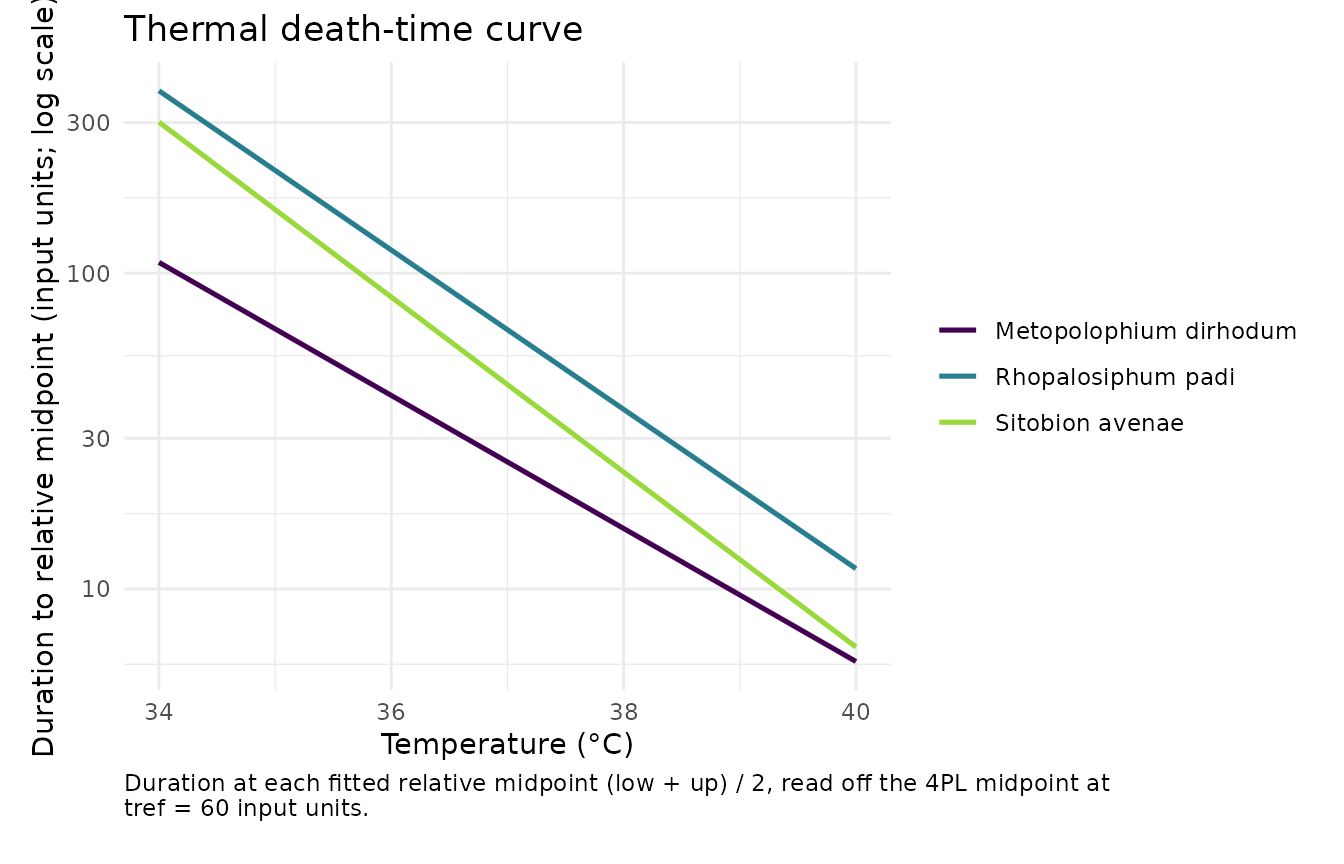

The table reports Wald confidence intervals. The TDT figure shows fitted point curves, not uncertainty intervals. Check convergence, Hessian status, gradient, and data-adequacy warnings before ranking species.

All-age heat extension

The supplement next uses all heat-branch ages and the direct fixed structure species * age on both headline coordinates. This is an experimental larger fixed-effect model in freqTLS; it is not a substitute empirical case.

aphid_all <- droplevels(subset(aphid_tdt, branch == "heat"))
aphid_all$species <- factor(
  aphid_all$species,
  levels = c("M_dirhodum", "R_padi", "S_avenae"),
  labels = c("Metopolophium dirhodum", "Rhopalosiphum padi",
             "Sitobion avenae")
)
aphid_all_std <- standardize_data(
  aphid_all, temp = "temp", duration = "duration_min",
  n_total = "n_total", n_surv = "n_surv", duration_unit = "minutes"
)
aphid_all_fit <- fit_4pl(
  aphid_all_std,
  ctmax = ~ 1 + species * age,
  z = ~ 1 + species * age,
  low = ~ 1,
  up = ~ 1,
  k = ~ temp_c,
  family = "beta_binomial",
  t_ref = 60,
  method = "wald",
  quiet = TRUE
)
diagnose_tdt_fit(aphid_all_fit)
#> # A tibble: 1 × 9
#>   converged pd_hessian max_abs_gradient gradient_pass optimizer  logLik n_params
#>   <lgl>     <lgl>                 <dbl> <lgl>         <chr>       <dbl>    <int>
#> 1 TRUE      TRUE              0.0000105 TRUE          nloptr_TN… -2303.       23
#> # ℹ 2 more variables: AIC <dbl>, all_pass <lgl>

The interacted formula coefficients are not themselves species-by-age values. The parameter prediction below evaluates the fitted direct coordinates for all nine biological cells at the observed mean assay temperature.

aphid_cells <- expand.grid(
  species = levels(aphid_all$species),
  age = levels(aphid_all$age),
  temp = mean(aphid_all_std$temp),
  KEEP.OUT.ATTRS = FALSE
)
aphid_cell_pars <- predict(aphid_all_fit, aphid_cells, type = "parameters")
cbind(aphid_cells[c("species", "age")],
      aphid_cell_pars[c("CTmax", "z")])
#>                  species age    CTmax        z
#> 1 Metopolophium dirhodum   2 35.10379 4.801607
#> 2     Rhopalosiphum padi   2 36.68836 3.384634
#> 3        Sitobion avenae   2 36.00785 4.169478
#> 4 Metopolophium dirhodum   6 35.22167 4.717234
#> 5     Rhopalosiphum padi   6 37.17018 3.842124
#> 6        Sitobion avenae   6 36.53607 3.564974
#> 7 Metopolophium dirhodum  12 35.99535 3.999057
#> 8     Rhopalosiphum padi  12 36.92917 3.890682
#> 9        Sitobion avenae  12 36.58300 3.275348

aphid_tdt_grid <- merge(
  expand.grid(
    temp = seq(min(aphid_all_std$temp), max(aphid_all_std$temp), length.out = 60),
    KEEP.OUT.ATTRS = FALSE
  ),
  aphid_cells[c("species", "age")]
)
aphid_tdt_pars <- predict(aphid_all_fit, aphid_tdt_grid, type = "parameters")
aphid_tdt_grid$duration_50 <- 10^(
  log10(60) - (aphid_tdt_grid$temp - aphid_tdt_pars$CTmax) / aphid_tdt_pars$z
)
ggplot2::ggplot(
  aphid_tdt_grid,
  ggplot2::aes(temp, duration_50, colour = species)
) +
  ggplot2::geom_line(linewidth = 0.8) +
  ggplot2::scale_y_log10() +
  ggplot2::facet_wrap(~ age) +
  ggplot2::labs(
    x = "Temperature (°C)",
    y = "Duration to 50% relative survival (minutes, log scale)",
    colour = "Species"
  ) +
  ggplot2::theme_minimal()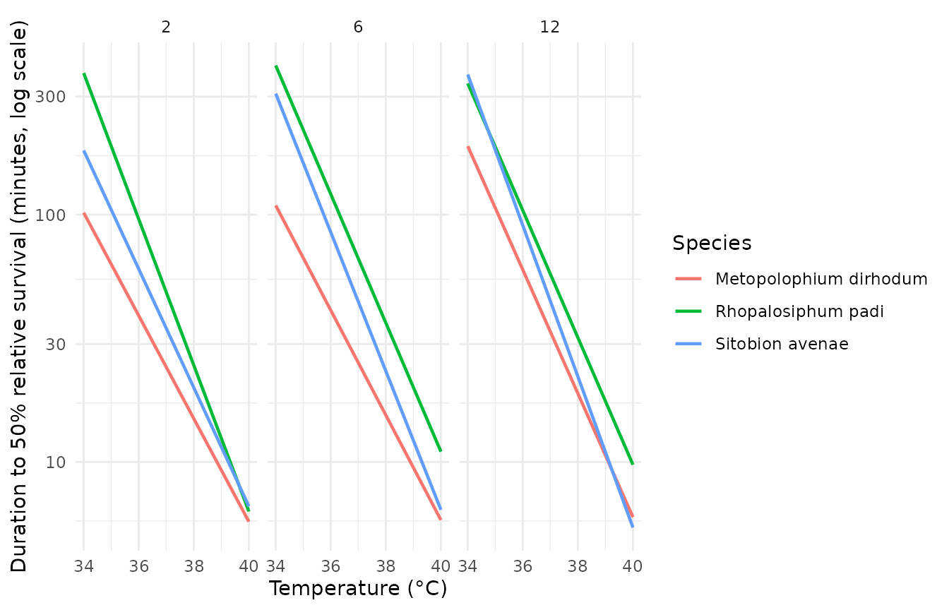

Projection boundary

The Wuhan field-temperature projection is not run here. Its environmental trace remains outside the installed package until the full redistribution chain is recorded in the licence ledger. predict_heat_injury() can evaluate a temperature trace, but any repair kernel supplied to current freqTLS is illustrative and unfitted. The fitted Bayesian projection remains available in bayesTLS.