Random effects: hierarchical thermal tolerance

This vignette is for a thermal biologist whose survival assays are grouped — colonies, clutches, populations, tanks, broods — and who wants to model between-group variation without spending a fixed coefficient on every group. That is exactly what a random intercept does: it treats the per-group deviations as draws from a Gaussian, estimates a single between-group standard deviation, and shrinks each group’s estimate toward the overall mean (partial pooling). In freqTLS a random intercept is available on the thermal-tolerance midpoint CTmax, the thermal-sensitivity log_z, and the shape coordinates low and log_k.

library(freqTLS)

Fixed groups vs. a random intercept

With a handful of well-sampled groups you can give each its own fixed CTmax (CTmax ~ group, see vignette("freqTLS")). With many groups — or groups you regard as a sample from a population — a random intercept CTmax ~ 1 + (1 | group) is the better tool: it costs one variance parameter instead of one coefficient per group, and the group estimates borrow strength from each other. The deviations b_g ~ N(0, sigma_CTmax^2) are integrated out by TMB’s Laplace approximation; sigma_CTmax is estimated by marginal maximum likelihood. A formula without (1 | group) uses the ordinary fixed-effects objective. Adding (1 | group) is not a no-op: it adds and integrates a group-level Gaussian block, even when its fitted variance is near zero.

A random intercept on CTmax

We simulate 14 colonies whose CTmax varies with a between-colony SD of 1.5 °C, then fit a single random intercept.

set.seed(1)
d <- simulate_tls(family = "binomial", CTmax = 36, z = 4,
                  re_sd = 1.5, n_re_groups = 14, seed = 1)
fit <- fit_tls(
  tls_bf(survived | trials(total) ~ time(duration) + temp(temp),
         CTmax ~ 1 + (1 | colony)),
  data = d, family = "binomial", tref = 1, quiet = TRUE)

# The estimates table carries the population CTmax / z and the between-colony SD.
est <- fit$estimates
est[est$parameter %in% c("CTmax", "z", "sigma_CTmax"),
    c("parameter", "estimate", "std.error")]
#>     parameter  estimate  std.error
#> 4       CTmax 36.010947 0.38977872
#> 5           z  3.952015 0.05042902
#> 6 sigma_CTmax  1.454802 0.27579903

sigma_CTmax is the estimated between-colony standard deviation of CTmax, in °C — directly interpretable on the thermal-tolerance scale. It is a maximum-likelihood variance component, so it is biased low when there are few groups: it is essentially unbiased by ~14 groups but increasingly shrunk toward zero below that. A focused recovery study makes the bias concrete and shows the fixed-effect CTmax interval losing coverage in step — the empirical basis for the advisory fit_tls() emits below ~8 groups. Repository maintainers can regenerate it with the source-only data-raw/re-recovery-study.R script, which is not installed:

Random-intercept recovery vs number of groups (true sigma_CTmax = 1.5; 150 sims/cell). The ML SD is biased low and the fixed-effect CTmax interval under-covers with few groups; both settle by ~14 groups.

n groups	mean sigma_CTmax	rel. bias	CTmax 95% coverage
3	1.044	-0.304	0.733
5	1.199	-0.200	0.853
8	1.352	-0.099	0.893
14	1.430	-0.047	0.933
30	1.448	-0.035	0.920

So with only a handful of groups the reported sigma_CTmax understates the true spread and the CTmax interval is optimistic. Prefer confint(method = "bootstrap") (or bayesTLS) for the fixed effects, and describe the variance component as likely downward-biased rather than treating it as a precise estimate or a literal confidence bound.

The conditional modes (BLUPs) — each colony’s shrunken deviation from the population CTmax — come from ranef():

head(ranef(fit), 4)
#> # A tibble: 4 × 4
#>   group term  estimate std.error
#>   <chr> <chr>    <dbl>     <dbl>
#> 1 g1    CTmax   -0.906     0.396
#> 2 g10   CTmax   -0.505     0.396
#> 3 g11   CTmax    2.16      0.396
#> 4 g12   CTmax    0.603     0.396

Prediction distinguishes the population curve from an observed colony’s conditional curve. Population predictions set the random intercept to zero; conditional predictions add the fitted BLUP and require the grouping column in newdata:

colony_1 <- as.character(ranef(fit)$group[1])
new_colony <- data.frame(temp = 36, duration = 2, colony = colony_1)
data.frame(
  target = c("population", "colony"),
  survival = c(
    predict(fit, new_colony, re.form = "population"),
    predict(fit, new_colony, re.form = "conditional")
  )
)
#>       target   survival
#> 1 population 0.19888224
#> 2     colony 0.08525094

Calling predict() without re.form on a random-effects fit warns and returns the population prediction. An unseen group cannot receive an estimated BLUP, so conditional prediction stops and points to re.form = "population".

confint() routes uncertainty by target. It gives a positive, log-scale Wald interval for sigma_CTmax. It profiles the population CTmax under the random effect, re-running the Laplace approximation at each grid point, so this is slower than a fixed-effects profile. If that fixed-effect profile does not close, the default fallback is Wald; request method = "bootstrap" to redraw the random effects and refit the full model instead.

suppressMessages(confint(fit, "sigma_CTmax", method = "wald"))[
  , c("parameter", "conf.low", "conf.high")]
#> # A tibble: 1 × 3
#>   parameter   conf.low conf.high
#>   <chr>          <dbl>     <dbl>
#> 1 sigma_CTmax     1.00      2.11
suppressMessages(confint(fit, "CTmax", method = "profile", npoints = 8))[
  , c("parameter", "conf.low", "conf.high", "method")]
#> # A tibble: 1 × 4
#>   parameter conf.low conf.high method 
#>   <chr>        <dbl>     <dbl> <chr>  
#> 1 CTmax         35.2      36.8 profile

The Confidence Eye always uses Wald intervals for a random-effects fit, even when method = "profile" is requested, because a profile eye would re-run the Laplace approximation at every grid point for every row. Use confint(fit, method = "profile") for fixed-effect profiles or confint(fit, method = "bootstrap") for random-effects-aware bootstrap intervals. The eye remains a confidence-interval display, never a posterior.

suppressMessages(plot_confidence_eye(fit, parm = "CTmax"))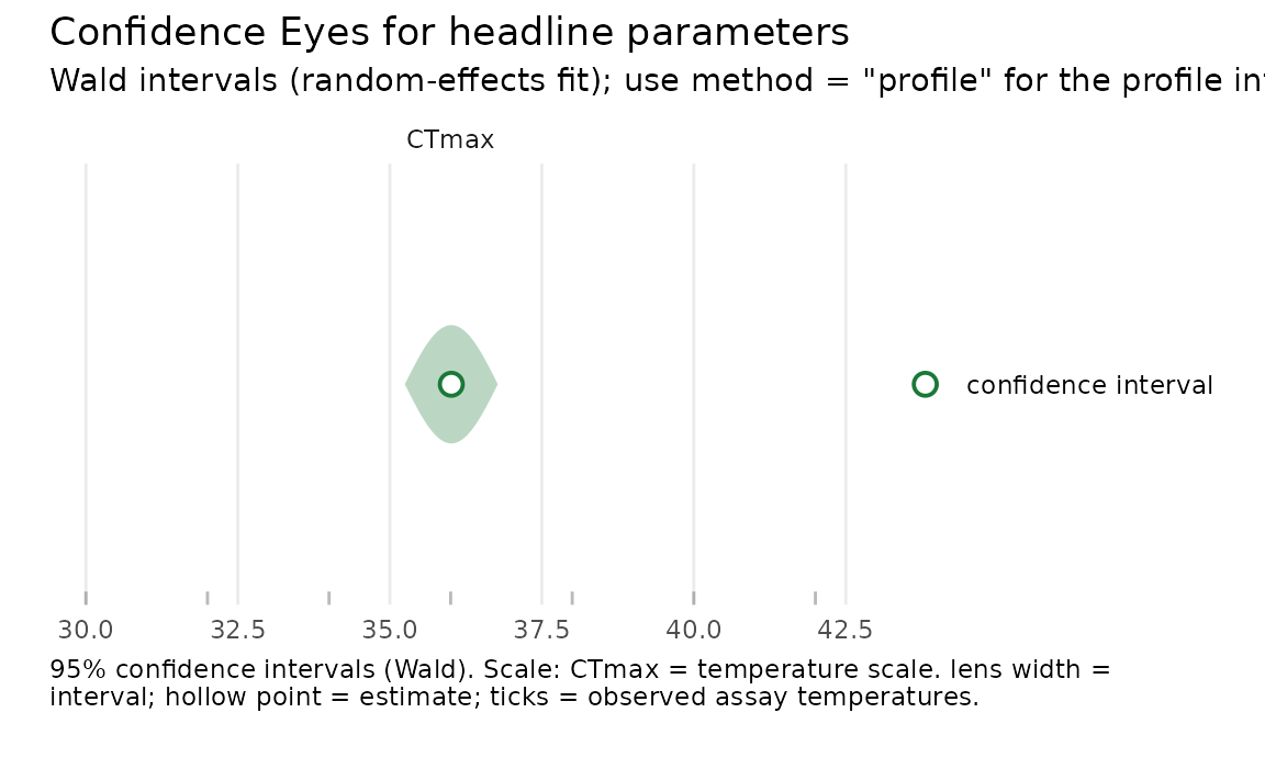

Random effects on sensitivity and curve shape

The same (1 | group) syntax works on log_z (thermal sensitivity) and on the shape coordinates low (the lower, long-exposure asymptote) and log_k (the steepness). One nuance matters: because z, low, and k are modelled on transformed scales, their variance components live on those scales — sigma_logz is a SD on log(z), sigma_low on logit(low), sigma_logk on log(k). Read sigma_logz as an approximate multiplicative spread on z: exp(sigma_logz) is the fold-change across groups, not a z-unit SD.

set.seed(2)
dz <- simulate_tls(family = "binomial", CTmax = 36, z = 4,
                   re_sd_z = 0.3, n_re_groups = 14, seed = 2)
fit_z <- fit_tls(
  tls_bf(survived | trials(total) ~ time(duration) + temp(temp),
         log_z ~ 1 + (1 | colony)),
  data = dz, family = "binomial", tref = 1, quiet = TRUE)
sg <- fit_z$estimates$estimate[fit_z$estimates$parameter == "sigma_logz"]
c(sigma_logz = round(sg, 3),
  approx_fold_spread_in_z = round(exp(sg), 3))
#>              sigma_logz approx_fold_spread_in_z 
#>                   0.265                   1.303

The upper asymptote up is the one shape with no random effect: under the disjoint-bounds parameterisation up = up_min + up_w * plogis(beta_up) it has its own coordinate beta_up, but the compiled objective carries no random-intercept term for up (and its profile path is not wired either — the same gap that leaves up with a delta-method interval). Put the random intercept on low or log_k instead.

Combining random effects, and what is out of scope

You can place random intercepts on more than one coordinate. When two or more share the same grouping factor, freqTLS fits them as independent variances (all cross-correlations forced to zero) and warns:

set.seed(3)
db <- simulate_tls(family = "binomial", CTmax = 36, z = 4,
                   re_sd = 1.2, re_sd_z = 0.3, n_re_groups = 14, seed = 3)
# Both random intercepts on the same `colony` grouping. This fits, but emits a
# warning that the two variances are independent (no correlation term); we pass
# `quiet = TRUE` to silence it here and discuss it below.
fit_both <- fit_tls(
  tls_bf(survived | trials(total) ~ time(duration) + temp(temp),
         CTmax ~ 1 + (1 | colony), log_z ~ 1 + (1 | colony)),
  data = db, family = "binomial", tref = 1, quiet = TRUE)
fit_both$estimates$parameter[grepl("^sigma", fit_both$estimates$parameter)]
#> [1] "sigma_CTmax" "sigma_logz"

In real data the group-level CTmax and z deviations are usually correlated; by forcing that correlation to zero, the independent-variance fit absorbs it into the marginal SDs and the fixed-effect intervals. If you need a correlated random effect — or crossed/nested grouping factors, or a random slope — use bayesTLS, whose Stan back end fits the full covariance. freqTLS deliberately stops at independent random intercepts on CTmax / log_z / low / log_k.

The likelihood view of shrinkage

A Gaussian random effect is a distributional model for the latent group deviations, not a prior placed on the reported population parameters. Its conditional modes (BLUPs) have an empirical-Bayes interpretation and shrink toward zero. The fixed effects and variance components are estimated by marginal maximum likelihood, and their intervals are profile-likelihood intervals for fixed-effect coordinates, log-scale Wald intervals for variance components, or parametric-bootstrap intervals when explicitly requested; they are not credible intervals. That is the same complementary stance the rest of freqTLS takes toward bayesTLS (see vignette("frequentist-and-bayesian")): the random effect buys you partial pooling without committing to priors on the parameters you report.