Case 4.2: Drosophila suzukii awake/coma response

Case 4.2 in the bayesTLS supplement contains several analyses. freqTLS supports only the awake/coma count arm. It does not replace the censored time-to-coma or hurdle-productivity models with a different endpoint.

library(freqTLS)
data(dsuzukii)

Exact awake-count aggregation

Within each temperature x exposure-level x sex cell, n_awake counts individuals that never entered coma (that is, they have no recorded t_coma). Duration is the first recorded time in the cell. Duration-zero controls are excluded because the 4PL uses log10(duration) and cannot represent zero duration; they are not evidence against up. Short positive exposures or mild treatments are the appropriate data for informing that upper asymptote.

cell <- interaction(dsuzukii$temp, dsuzukii$lvl, dsuzukii$sex, drop = TRUE)
coma <- do.call(rbind, lapply(split(dsuzukii, cell), function(d) {
  data.frame(
    temp = d$temp[1], lvl = d$lvl[1], sex = d$sex[1],
    duration = d$time[1], n_total = nrow(d),
    n_awake = sum(is.na(d$t_coma))
  )
}))
coma <- droplevels(subset(coma, duration > 0))
coma_std <- standardize_data(
  coma, temp = "temp", duration = "duration",
  n_total = "n_total", n_surv = "n_awake", duration_unit = "minutes"
)

Locked model

The awake/coma response is beta-binomial. The direct headline formulas retain an intercept (~ sex), while low, up, and k each vary with centred assay temperature. The reference is 60 minutes and the estimand is the relative midpoint.

coma_fit <- fit_4pl(
  coma_std,
  ctmax = ~ sex,
  z = ~ sex,
  low = ~ temp_c,
  up = ~ temp_c,
  k = ~ temp_c,
  family = "beta_binomial",
  t_ref = 60,
  method = "wald",
  quiet = TRUE
)
diagnose_tdt_fit(coma_fit)
#> # A tibble: 1 × 9
#>   converged pd_hessian max_abs_gradient gradient_pass optimizer logLik n_params
#>   <lgl>     <lgl>                 <dbl> <lgl>         <chr>      <dbl>    <int>
#> 1 TRUE      TRUE              0.0000120 TRUE          nlminb     -130.       11
#> # ℹ 2 more variables: AIC <dbl>, all_pass <lgl>
check_tls(coma_fit)

The lower-asymptote coefficients are weakly identified even though the optimizer, Hessian, and raw-gradient checks pass. The actual estimates and standard errors make that limitation visible.

coma_shape <- subset(
  coma_fit$fit$estimates,
  grepl("^(low|up|k):", parameter),
  select = c(parameter, estimate, std.error)
)
coma_shape
#>         parameter    estimate    std.error
#> 1 low:(Intercept) -44.2916768 1.781037e+04
#> 2      low:temp_c -20.2774545 8.455428e+03
#> 3  up:(Intercept)   2.6835505 8.010875e-01
#> 4       up:temp_c   0.4135033 4.957870e-01
#> 5   k:(Intercept)   2.7540874 1.471270e-01
#> 6        k:temp_c  -0.2713143 9.005695e-02

coma_table <- tls(coma_fit, by = "sex", lethal = FALSE, method = "wald")$summary
names(coma_table)[names(coma_table) == "median"] <- "estimate"
coma_table
#> # A tibble: 4 × 5
#>   sex   quantity estimate lower upper
#>   <chr> <chr>       <dbl> <dbl> <dbl>
#> 1 F     CTmax       36.5  36.4  36.6 
#> 2 M     CTmax       36.3  36.2  36.4 
#> 3 F     z            2.43  2.29  2.59
#> 4 M     z            2.39  2.26  2.53

Only CTmax and z are reported; Tcrit is not. The output returns large shape-coefficient standard errors and warnings for transparency.

plot_survival_curves(coma_fit$fit)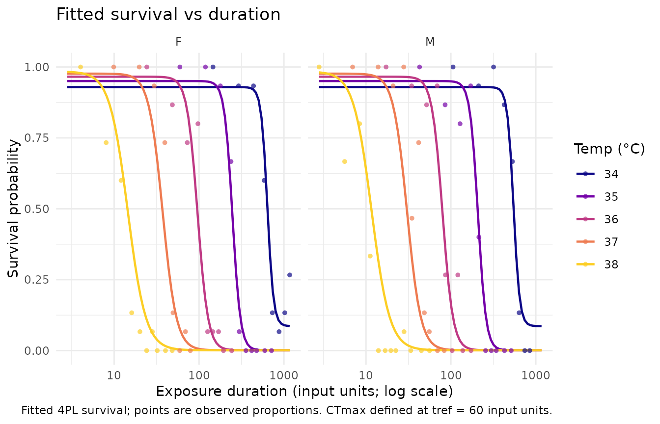

Unsupported arms

The individual t_coma values form a censored time-to-event outcome, and prod requires a hurdle model for zero reproduction plus positive clutch size. freqTLS 0.1.0 implements neither. Use the corresponding bayesTLS Case 4.2 sections for those analyses rather than treating the count model above as a replacement.