From Raw Data to PCM: A Complete Bird Trait Workflow
Source:vignettes/bird-workflow.Rmd
bird-workflow.RmdThis vignette walks through a real comparative biology workflow using avian trait data and a phylogenetic tree. The same approach applies to any taxon group — mammals, fish, amphibians, plants — the functions are fully taxon-agnostic.
Part I: Core Workflow
The typical workflow has four steps: load your data and tree, reconcile the names, produce aligned objects, and run your analysis.
Step 1: Load data and tree
data(avonet_subset)    # AVONET morphological traits (Tobias et al. 2022)
data(tree_jetz)    # Jetz et al. (2012) phylogeny, Corvoidea + allies

cat(sprintf("Data: %d species\n", nrow(avonet_subset)))
#> Data: 919 species
cat(sprintf("Tree: %d tips\n", ape::Ntip(tree_jetz)))
#> Tree: 657 tips

# The data uses spaces; the tree uses underscores
head(avonet_subset$Species1, 3)
#> [1] "Acanthiza apicalis"    "Acanthiza chrysorrhoa" "Acanthiza cinerea"
head(tree_jetz$tip.label, 3)
#> [1] "Amytornis_barbatus"  "Amytornis_merrotsyi" "Amytornis_dorotheae"
These formatting differences — spaces vs underscores, minor spelling variants, taxonomic synonyms — are exactly what prepR4pcm resolves.
Step 2: Reconcile data against the tree
result <- reconcile_tree(
  x = avonet_subset,
  tree = tree_jetz,
  x_species = "Species1",
  authority = NULL       # skip synonym lookup for speed
)
#> ℹ Reconciling 919 data names vs 657 tree tips
#> ℹ Matching 919 x 657 names through 2 stages...
#> ℹ Stage 1/2: Exact matching...
#> ℹ Stage 2/2: Normalised matching (0 matched so far)...
#> ✔ Matched 657/919 data names to tree tips
print(result)
#>
#> ── Reconciliation: data vs tree ────────────────────────────────────────────────
#>   Source x: avonet_subset
#>   Source y: phylo (657 tips)
#>   Authority: none
#>   Timestamp: 2026-06-16 10:10:09
#> ℹ Match coverage: [█████████████████████░░░░░░░░░] 71% (657/919)
#>
#> ── Match summary ──
#>
#> • Exact: 0 ( 0.0%)
#> • Normalized: 657 (71.5%)
#> • Synonym: 0 ( 0.0%)
#> • Fuzzy: 0 ( 0.0%)
#> • Manual: 0 ( 0.0%)
#> ! Unresolved (x only):262 (28.5%)
#> ! Unresolved (y only):0
#> ! Flagged for review: 0
#> ℹ Use `reconcile_summary()` for details, `reconcile_mapping()` for the full table.
The reconciliation object records every name-matching decision. Inspect the mapping to see what happened:
mapping <- reconcile_mapping(result)

# Match type breakdown
table(mapping$match_type)
#>
#> normalized unresolved
#>        657        262

# Show normalised matches (formatting differences resolved automatically)
norm <- mapping[mapping$match_type == "normalized",
                c("name_x", "name_y", "notes")]
if (nrow(norm) > 0) head(norm, 5)
#> # A tibble: 5 × 3
#>   name_x                name_y                notes
#>   <chr>                 <chr>                 <chr>
#> 1 Acanthiza apicalis    Acanthiza_apicalis    'Acanthiza apicalis' normalised t…
#> 2 Acanthiza chrysorrhoa Acanthiza_chrysorrhoa 'Acanthiza chrysorrhoa' normalise…
#> 3 Acanthiza ewingii     Acanthiza_ewingii     'Acanthiza ewingii' normalised to…
#> 4 Acanthiza inornata    Acanthiza_inornata    'Acanthiza inornata' normalised t…
#> 5 Acanthiza iredalei    Acanthiza_iredalei    'Acanthiza iredalei' normalised t…

# Unresolved: in data but not in tree
unresolved <- mapping[mapping$match_type == "unresolved" & mapping$in_x, ]
cat(sprintf("\nSpecies in data but not in tree: %d\n", nrow(unresolved)))
#>
#> Species in data but not in tree: 262
For a detailed report:
reconcile_summary(result, detail = "mismatches_only")Step 3: Produce aligned objects
Drop unresolved species to get a matched data frame and tree, ready for comparative analysis:
aligned <- reconcile_apply(
  result,
  data = avonet_subset,
  tree = tree_jetz,
  species_col = "Species1",
  drop_unresolved = TRUE
)
#> ! Dropped 262 rows with unresolved species from data
#> ℹ Tree has 657 tips after alignment

cat(sprintf("Aligned data: %d rows\nAligned tree: %d tips\n",
            nrow(aligned$data), ape::Ntip(aligned$tree)))
#> Aligned data: 657 rows
#> Aligned tree: 657 tips
Step 4: Run a comparative analysis
With aligned data and tree, you are ready for any phylogenetic comparative method. Here are two common approaches.
Phylogenetic generalised least squares (PGLS)
PGLS accounts for shared evolutionary history when estimating regression parameters:
library(caper)

# reconcile_apply() aligns names so data$Species1 matches tree tip labels
cd <- comparative.data(aligned$tree, aligned$data,
                       names.col = "Species1", vcv = TRUE)

# PGLS: body mass ~ wing length
model_pgls <- pgls(log(Mass) ~ log(Wing.Length), data = cd)
summary(model_pgls)
#>
#> Call:
#> pgls(formula = log(Mass) ~ log(Wing.Length), data = cd)
#>
#> Residuals:
#>      Min       1Q   Median       3Q      Max
#> -0.53264 -0.04823 -0.00130  0.04332  0.50941
#>
#> Branch length transformations:
#>
#> kappa  [Fix]  : 1.000
#> lambda [Fix]  : 1.000
#> delta  [Fix]  : 1.000
#>
#> Coefficients:
#>                   Estimate Std. Error t value  Pr(>|t|)
#> (Intercept)      -5.781917   0.381775 -15.145 < 2.2e-16 ***
#> log(Wing.Length)  2.054361   0.065135  31.540 < 2.2e-16 ***
#> ---
#> Signif. codes:  0 '***' 0.001 '**' 0.01 '*' 0.05 '.' 0.1 ' ' 1
#>
#> Residual standard error: 0.09582 on 651 degrees of freedom
#> Multiple R-squared: 0.6044,  Adjusted R-squared: 0.6038
#> F-statistic: 994.8 on 1 and 651 DF,  p-value: < 2.2e-16
Phylogenetic generalised linear mixed model (PGLMM)
When you need random effects beyond phylogeny or want a Bayesian framework, use a PGLMM. The MCMCglmm package fits Bayesian phylogenetic mixed models:
library(MCMCglmm)

# Species column as the phylogenetic grouping factor
aligned$data$phylo <- aligned$data$Species1

# Inverse phylogenetic covariance matrix
# Replace any zero-length branches (can arise after pruning)
tree_mcmc <- aligned$tree
tree_mcmc$edge.length[tree_mcmc$edge.length < .Machine$double.eps] <- 1e-6
inv_phylo <- inverseA(tree_mcmc, nodes = "ALL", scale = FALSE)

# PGLMM: continuous response
prior <- list(R = list(V = 1, nu = 0.002),
              G = list(G1 = list(V = 1, nu = 0.002)))

model_mcmc <- MCMCglmm(
  log(Mass) ~ log(Wing.Length) + Trophic.Level,
  random = ~phylo,
  family = "gaussian",
  ginverse = list(phylo = inv_phylo$Ainv),
  data = aligned$data,
  prior = prior,
  nitt = 50000, burnin = 10000, thin = 20,
  verbose = FALSE
)
summary(model_mcmc)
#>
#>  Iterations = 10001:49981
#>  Thinning interval  = 20
#>  Sample size  = 2000
#>
#>  DIC: -177.321
#>
#>  G-structure:  ~phylo
#>
#>       post.mean l-95% CI u-95% CI eff.samp
#> phylo   0.00168 0.001246 0.002134     1357
#>
#>  R-structure:  ~units
#>
#>       post.mean l-95% CI u-95% CI eff.samp
#> units    0.0316  0.02657  0.03692     1555
#>
#>  Location effects: log(Mass) ~ log(Wing.Length) + Trophic.Level
#>
#>                        post.mean l-95% CI u-95% CI eff.samp  pMCMC
#> (Intercept)             -6.23721 -6.77124 -5.74511     1916 <5e-04 ***
#> log(Wing.Length)         2.15198  2.04803  2.25511     1829 <5e-04 ***
#> Trophic.LevelHerbivore   0.02755 -0.05682  0.10939     2000  0.518
#> Trophic.LevelOmnivore    0.03632 -0.03227  0.10284     2000  0.271
#> ---
#> Signif. codes:  0 '***' 0.001 '**' 0.01 '*' 0.05 '.' 0.1 ' ' 1
For categorical responses (e.g., migration status with multiple categories), see Mizuno et al. (2025, J. Evol. Biol. 38:1699–1715) for the multinomial PGLMM approach and the accompanying tutorial at https://ayumi-495.github.io/multinomial-GLMM-tutorial/.
See Hadfield (2010, J. Stat. Softw. 33:1–22) for MCMCglmm details, Hadfield & Nakagawa (2010, J. Evol. Biol. 23:494–508) for phylogenetic quantitative genetics, and Mizuno et al. (2025, J. Evol. Biol. 38:1699–1715) for phylogenetic multinomial mixed models.
That is the complete core workflow: load, reconcile, apply, analyse.
Part II: Advanced Topics
Reconciling two datasets
If you need to harmonise species names across two trait datasets
before matching to a tree, use
reconcile_data():
data(nesttrait_subset)   # Nest traits (Chia et al. 2023)

rec_data <- reconcile_data(
  x = nesttrait_subset,
  y = avonet_subset,
  x_species = "Scientific_name",
  y_species = "Species1",
  authority = NULL,
  quiet = TRUE
)
print(rec_data)
#>
#> ── Reconciliation: data vs data ────────────────────────────────────────────────
#>   Source x: nesttrait_subset
#>   Source y: avonet_subset
#>   Authority: none
#>   Timestamp: 2026-06-16 10:10:28
#> ℹ Match coverage: [██████████████████████████████] 100% (916/916)
#>
#> ── Match summary ──
#>
#> • Exact: 916 (100.0%)
#> • Normalized: 0 ( 0.0%)
#> • Synonym: 0 ( 0.0%)
#> • Fuzzy: 0 ( 0.0%)
#> • Manual: 0 ( 0.0%)
#> ! Unresolved (x only):0 ( 0.0%)
#> ! Unresolved (y only):3
#> ! Flagged for review: 0
#> ℹ Use `reconcile_summary()` for details, `reconcile_mapping()` for the full table.
Once reconciled, merge the two datasets into a single data frame:
merged <- reconcile_merge(
  rec_data,
  data_x = nesttrait_subset,
  data_y = avonet_subset,
  species_col_x = "Scientific_name",
  species_col_y = "Species1"
)
#> ✔ Merged 916 species (inner join)
cat(sprintf("Merged: %d rows, %d columns\n", nrow(merged), ncol(merged)))
#> Merged: 916 rows, 31 columns
Multi-row species
reconcile_merge() assumes one row per species in each
data frame. If a species appears in multiple rows (e.g. sex-specific
measurements, repeated populations, or individual-level records), the
merge produces all pairwise combinations for that species — the same
behaviour as base merge(). reconcile_merge()
warns when it detects duplicates so that you are not surprised by row
expansion.
There are two sensible ways to handle multi-row data:
Option A. Aggregate first, merge second. If your downstream PCM expects one row per species (most PGLS and PGLMM workflows do), collapse to a species-level summary before merging:
# Example: averaging individual measurements to species means
species_means <- aggregate(
  cbind(Mass, Wing.Length) ~ Species1,
  data = individual_measurements,
  FUN  = mean
)
merged <- reconcile_merge(rec_data, species_means, avonet_subset,
                          species_col_x = "Species1",
                          species_col_y = "Species1")
Option B. Reconcile once, join the mapping back to the full data. If you want to keep every row (e.g. for an individual-level PGLMM), build the reconciliation on a species-level summary and then use the mapping as a lookup table for the original, multi-row data:
# Reconcile on unique species
species_level <- data.frame(
  Species1 = unique(individual_measurements$Species1)
)
rec <- reconcile_data(species_level, avonet_subset,
                      x_species = "Species1", y_species = "Species1",
                      authority = NULL, quiet = TRUE)

# Join the mapping back to the full, multi-row dataset
mapping <- reconcile_mapping(rec)
individual_measurements$species_resolved <- mapping$name_resolved[
  match(individual_measurements$Species1, mapping$name_x)
]
Asymmetric datasets
A common situation in comparative biology is merging a small focal
dataset against a much larger reference (e.g. a field study of 50
species against AVONET’s ~10,000). reconcile_merge()
accepts datasets of any size, but the how argument
matters:
# Keep only species present in both: inner join
inner <- reconcile_merge(rec_data, small_data, large_data,
                         species_col_x = "species",
                         species_col_y = "Species1",
                         how = "inner")

# Keep all small_data rows; fill large_data columns with NA
# for species missing from the reference: left join
left <- reconcile_merge(rec_data, small_data, large_data,
                        species_col_x = "species",
                        species_col_y = "Species1",
                        how = "left")
Use how = "inner" when the analysis cannot tolerate
NAs in the reference columns, and how = "left"
when you want to retain every focal-study species (and you will handle
missingness in the model). how = "full" is rarely what you
want here — it would return the entire reference dataset padded with
NAs for every focal trait.
Using a taxonomy crosswalk
When your data and tree use different taxonomies (e.g., BirdLife data against a BirdTree phylogeny), a curated crosswalk can resolve names that automated synonym resolution misses.
A crosswalk is simply a table mapping names from one system to another. prepR4pcm includes the BirdLife-BirdTree crosswalk as an example:
data(crosswalk_birdlife_birdtree)
table(crosswalk_birdlife_birdtree$Match.type)
#>
#>              1BL to 1BT          1BL to many BT                 Extinct
#>                    8960                     225                     143
#>          Many BL to 1BT Newly described species
#>                    1933                      24
Convert it to an overrides table and pass it to
reconcile_tree():
overrides <- reconcile_crosswalk(
  crosswalk_birdlife_birdtree,
  from_col = "Species1",
  to_col = "Species3",
  match_type_col = "Match.type"
)
#> ℹ 1933 many-to-one entries (lumps) included
#> ℹ 225 one-to-many entries (splits) included
#> ✔ Crosswalk: 3039 overrides (8079 identical pairs skipped)

# Re-reconcile with overrides
result_xw <- reconcile_tree(
  x = avonet_subset,
  tree = tree_jetz,
  x_species = "Species1",
  authority = NULL,
  overrides = overrides
)
#> ℹ Reconciling 919 data names vs 657 tree tips
#> ℹ Matching 919 x 657 names through 2 stages...
#> ℹ Stage 1/2: Exact matching...
#> ℹ Stage 2/2: Normalised matching (68 matched so far)...
#> ! 2971 overrides could not be applied: 23 already_matched; 2767 name_x_not_in_data; 181 name_y_not_in_target.
#> ℹ See `result$unused_overrides` for details.
#> ✔ Matched 657/919 data names to tree tips

# Compare: how many more matches with the crosswalk?
cat(sprintf("Without crosswalk: %d matched\n",
            sum(result$mapping$in_x & result$mapping$in_y, na.rm = TRUE)))
#> Without crosswalk: 657 matched
cat(sprintf("With crosswalk:    %d matched\n",
            sum(result_xw$mapping$in_x & result_xw$mapping$in_y, na.rm = TRUE)))
#> With crosswalk:    657 matched
When do you need a crosswalk? Only when your data and tree follow different naming authorities and a curated mapping exists. For most use cases, the automatic cascade (exact → normalised → synonym) is sufficient.
You can also build your own overrides manually — it is just a data
frame with name_x, name_y, and optionally
user_note columns:
my_overrides <- data.frame(
  name_x    = c("Old name A", "Old name B"),
  name_y    = c("Tree name A", "Tree name B"),
  user_note = c("Reclassified in 2023", "Spelling correction")
)
result <- reconcile_tree(my_data, my_tree, overrides = my_overrides)
Reconciling against multiple trees
For sensitivity analyses across phylogenies,
reconcile_to_trees() reconciles one dataset against several
trees in one call:
data(tree_clements25)  # Clements 2025 tree

results <- reconcile_to_trees(
  x = avonet_subset,
  trees = list(
    jetz      = tree_jetz,
    clements  = tree_clements25
  ),
  x_species = "Species1",
  authority = NULL
)
#> ℹ Reconciling 919 data names against 2 trees
#> ℹ   [jetz] 657 tips
#> ℹ Matching 919 x 657 names through 2 stages...
#> ℹ Stage 1/2: Exact matching...
#> ℹ Stage 2/2: Normalised matching (0 matched so far)...
#> ✔   [jetz] Matched 657/919 names
#> ℹ   [clements] 854 tips
#> ℹ Matching 919 x 854 names through 2 stages...
#> ℹ Stage 1/2: Exact matching...
#> ℹ Stage 2/2: Normalised matching (0 matched so far)...
#> ✔   [clements] Matched 854/919 names

# Compare overlap across trees
sapply(results, function(r) {
  c(matched = sum(r$mapping$in_x & r$mapping$in_y, na.rm = TRUE),
    unresolved_x = r$counts$n_unresolved_x)
})
#>              jetz clements
#> matched       657      854
#> unresolved_x  262       65
Fuzzy matching for typos
Enable fuzzy matching to catch likely typos in species names:
result <- reconcile_tree(
  x = my_data,
  tree = my_tree,
  fuzzy = TRUE,              # enable fuzzy matching
  fuzzy_threshold = 0.9,     # minimum similarity (0-1)
  resolve = "flag"           # flag low-confidence matches for review
)

# Check flagged matches
flagged <- reconcile_mapping(result)
flagged[flagged$match_type == "flagged", c("name_x", "name_y", "match_score")]
Tree augmentation for missing species
When the tree has fewer species than the data,
reconcile_apply() drops the unresolved species. This loses
statistical power and can bias the sample.
reconcile_augment() grafts the missing species onto the
tree using genus-level placement:
aug <- reconcile_augment(
  result,
  tree_jetz,
  where = "genus",                # sister to a random congener
  branch_length = "congener_median",  # median terminal branch of congeners
  seed = 42,                      # for reproducibility
  quiet = TRUE
)
#> Warning: Tree returned by "internal" is not strictly ultrametric.
#> ℹ Most PCM methods (PGLS, BM, OU, etc.) assume ultrametric trees.
#> → To force: `phytools::force.ultrametric(result$tree)` or
#>   `ape::chronos(result$tree)`.
#> • To suppress this check: pass `check_ultrametric = FALSE`.

cat(sprintf("Original tips: %d\nAugmented tips: %d\n",
            ape::Ntip(aug$original), ape::Ntip(aug$tree)))
#> Original tips: 657
#> Augmented tips: 793
cat(sprintf("Added: %d | Skipped (no congener): %d\n",
            nrow(aug$augmented), nrow(aug$skipped)))
#> Added: 136 | Skipped (no congener): 126

# Which species were added, and where?
if (nrow(aug$augmented) > 0) head(aug$augmented[, c("species", "placed_near", "branch_length")])
#> # A tibble: 6 × 3
#>   species                  placed_near             branch_length
#>   <chr>                    <chr>                           <dbl>
#> 1 Acanthiza cinerea        Acanthiza lineata                5.04
#> 2 Calamanthus cautus       Calamanthus fuliginosus          3.80
#> 3 Calamanthus montanellus  Calamanthus fuliginosus          3.80
#> 4 Calamanthus pyrrhopygius Calamanthus fuliginosus          3.80
#> 5 Gerygone citrina         Gerygone magnirostris            2.91
#> 6 Pyrrholaemus sagittatus  Pyrrholaemus brunneus           15.5
Use the augmented tree in downstream analyses. Pass the augmented
tree to reconcile_apply() — the existing reconciliation
object is still valid as the name-mapping key, but the new tree contains
the extra tips, so drop_unresolved = FALSE retains the
grafted species:
aligned_aug <- reconcile_apply(
  result,
  data = avonet_subset,
  tree = aug$tree,        # augmented tree, not the original
  species_col = "Species1",
  drop_unresolved = FALSE  # keep augmented tips (they are now in the tree)
)
Important caveat. Genus-level placement assumes the
missing species diverged similarly to its congeners, which may not hold.
Always report which species were augmented (aug$augmented)
and run sensitivity analyses comparing results with and without
them.
Exporting to files
Write aligned data, tree, and the full mapping table to disk:
reconcile_export(
  result,
  data = avonet_subset,
  tree = tree_jetz,
  species_col = "Species1",
  dir = "output",
  prefix = "avonet_jetz"
)
# Writes: avonet_jetz_data.csv, avonet_jetz_tree.nex, avonet_jetz_mapping.csv
HTML reports
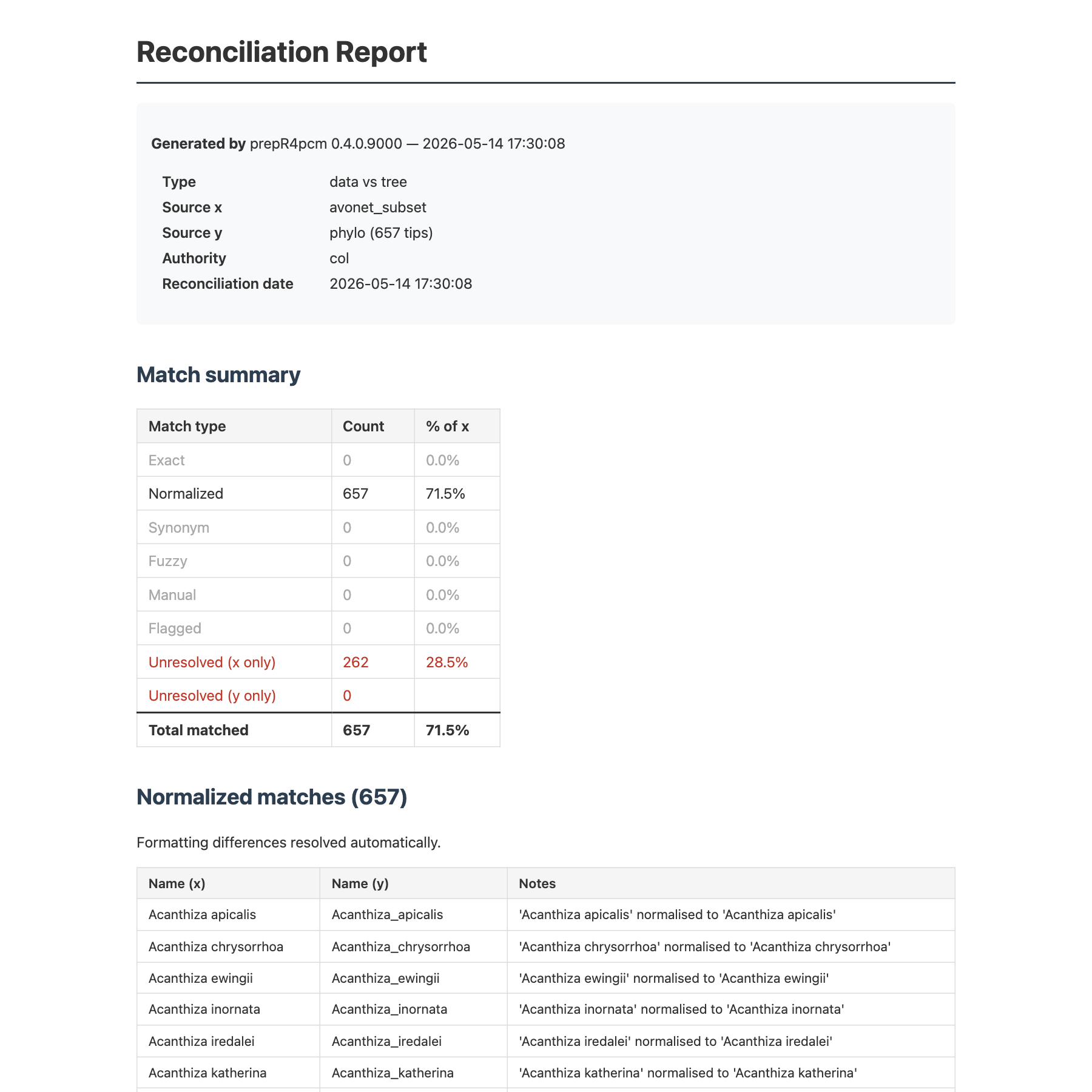
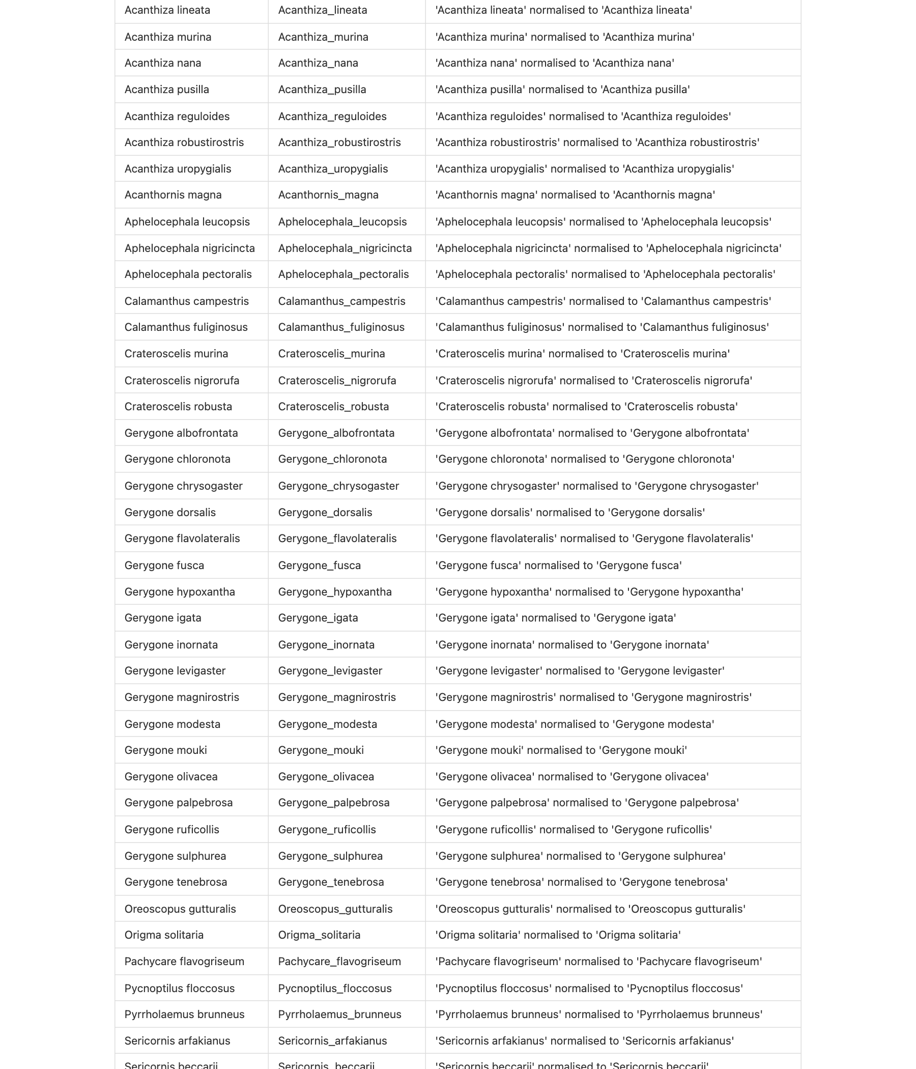
Generate a self-contained HTML report documenting every name-matching decision. Useful for sharing with collaborators or archiving alongside your analysis:
reconcile_report(result, file = "reconciliation_report.html")The report opens in any browser. It begins with the run header, match-coverage summary, and a small bar chart of match composition (Figure 1). Further down, per-match-type detail tables and the unresolved-species list make each decision auditable (Figure 2). The file is self-contained — styles, charts, and tables are all inline — so it can be archived or shared without external assets.
Key points
Taxon-agnostic. This workflow works for any group — mammals, fish, amphibians, plants — as long as you have a data frame and a phylogenetic tree.
Provenance. Every name-matching decision is recorded in the
reconciliationobject. Usereconcile_summary()for a human-readable report orreconcile_mapping()for the full table.Crosswalks are optional. Most users do not need them. The automatic cascade handles formatting differences and synonyms. Crosswalks help when two well-known naming authorities disagree.
Tree augmentation. When the tree is incomplete,
reconcile_augment()grafts missing species using congener placement — but always run sensitivity analyses with and without augmented tips.Sensitivity.
reconcile_to_trees()makes it easy to run the same analysis across multiple phylogenies.Merging.
reconcile_merge()joins two reconciled datasets into a single analysis-ready data frame, using the mapping as the join key.Reports.
reconcile_report()generates a self-contained HTML report suitable for sharing or archiving.Visualisation.
reconcile_plot()produces a bar or pie chart of match composition.reconcile_suggest()shows the closest fuzzy candidates for unresolved species.Comparison.
reconcile_diff()compares two reconciliation runs side by side — e.g., before and after adding a crosswalk.
Data sources
- AVONET: Tobias et al. (2022) Ecology Letters 25:581–597. DOI 10.1111/ele.13898
- NestTrait v2: Chia et al. (2023) Scientific Data 10:923. DOI 10.1038/s41597-023-02837-1
- Plumage lightness: Delhey et al. (2019) Ecology Letters 22:726–736. DOI 10.1111/ele.13233
- Jetz tree: Jetz et al. (2012) Nature 491:444–448. DOI 10.1038/nature11631
- Clements 2025: Clements et al. (2025) eBird/Clements Checklist.
- BirdLife-BirdTree crosswalk: Tobias et al. (2022).
References
- Hadfield, J.D. (2010) MCMC methods for multi-response generalized linear mixed models: the MCMCglmm R package. Journal of Statistical Software 33:1–22. DOI 10.18637/jss.v033.i02
- Hadfield, J.D. & Nakagawa, S. (2010) General quantitative genetic methods for comparative biology: phylogenies, taxonomies and multi-trait models for continuous and categorical characters. Journal of Evolutionary Biology 23:494–508. DOI 10.1111/j.1420-9101.2009.01915.x
- Mizuno, A., Drobniak, S.M., Williams, C., Lagisz, M. & Nakagawa,
S.
- Promoting the use of phylogenetic multinomial generalised mixed-effects model to understand the evolution of discrete traits. Journal of Evolutionary Biology 38:1699–1715. DOI 10.1093/jeb/voaf116. Tutorial: https://ayumi-495.github.io/multinomial-GLMM-tutorial/
- Norman, K.E., Chamberlain, S. & Boettiger, C. (2020) taxadb: A high-performance local taxonomic database interface. Methods in Ecology and Evolution 11:1153–1159. DOI 10.1111/2041-210X.13440
- Orme, D., Freckleton, R., Thomas, G., Petzoldt, T., Fritz, S., Isaac, N. & Pearse, W. (2025) caper: Comparative Analyses of Phylogenetics and Evolution in R. R package version 1.0.4. DOI 10.32614/CRAN.package.caper
- Paradis, E. & Schliep, K. (2019) ape 5.0: an environment for modern phylogenetics and evolutionary analyses in R. Bioinformatics 35:526–528. DOI 10.1093/bioinformatics/bty633