Phylogenetic meta-analysis with rotl + prepR4pcm

Phylogenetic meta-analysis is the dominant comparative workflow in ecology and evolutionary biology when the dataset spans many higher taxa: you compute an effect size per study, then fit a model that controls for shared evolutionary history.

The standard recipe (Cinar et al. 2022, Methods Ecol. Evol. 13:383) looks like:

Pull a topology from Open Tree of Life via rotl. Open Tree of Life gives you tip labels and branching structure; the edge lengths it returns are unit-length placeholders — not biologically meaningful time/divergence values.
Resolve polytomies at random via ape::multi2di(random = TRUE). The phylogenetic correlation matrix you’ll feed into the meta-analysis model has to be full-rank, which means strictly bifurcating.
Assign branch lengths via Grafen’s (1989) method: ape::compute.brlen(tree, method = "Grafen"). Grafen’s method is the canonical choice for meta-analysis when no time-calibrated branches are available.
Compute the phylogenetic correlation matrix: ape::vcv(tree, corr = TRUE).
Fit the meta-analysis with metafor::rma.mv() (or MCMCglmm, brms, glmmTMB, etc.) using the correlation matrix as a random-effect structure.

prepR4pcm wraps steps 1-3 into a single pr_get_tree() call, and step 4 into a single pr_phylo_cor() call. This vignette walks through the whole pipeline.

A worked example: thermal-tolerance plasticity across animal classes

We’ll mirror the phylogeny construction from Pottier et al. (2022) “Developmental plasticity in thermal tolerance” (Ecology Letters 25(10):2245-2268, DOI 10.1111/ele.14083). Their dataset spans 147 ectotherm species across 14 animal classes — fish, insects, reptiles, amphibians, crustaceans, bivalves, echinoderms, cephalopods, etc.

This is the cross-taxon case where rotl is the only practical option for retrieval. The taxon-specific mega-tree backends (the external tree-source packages that pr_get_tree() draws on) each cover one clade only: rtrees ships separate mega-trees for mammals, birds, fish, amphibians, squamates and a handful of other taxa; fishtree covers ray-finned fish only; clootl covers birds only. None of those backends spans the 14-class breadth of an ectotherm meta-analysis. The Open Tree of Life is a synthetic tree (i.e. a composite made by merging other trees). Parameter source = "rotl" from the prepR4pcm package function pr_get_tree() returns a single tree spanning every class in the dataset, without branch lengths.

Setup

We will use three packages: prepR4pcm (this package, for the retrieve / clean / correlate pipeline), rotl (the Open Tree of Life client that pr_get_tree(source = "rotl") calls under the hood), and metafor (the meta-analysis engine that consumes the phylogenetic correlation matrix).

library(prepR4pcm)
# install.packages("rotl")     # required: Open Tree of Life access
# install.packages("metafor")  # required: the meta-analysis engine

Step 1-3: topology -> bifurcating -> Grafen branches, in one call

For brevity we use 14 representative species — one or two from each major class in the Pottier dataset. Each class label below points at one or two species drawn from a different chunk of the ectotherm tree. We picked these classes because they are the ones contributing the most studies in Pottier et al. (2022); a real analysis would use all 147 species from the Pottier dataset.

species <- c(
  # Actinopterygii (ray-finned fish)
  "Salmo trutta",              "Acipenser fulvescens",
  # Reptilia
  "Anolis sagrei",
  # Amphibia
  "Xenopus laevis",            "Rhinella marina",
  # Insecta
  "Ischnura elegans",          "Anopheles albimanus",
  # Malacostraca (crustaceans)
  "Litopenaeus vannamei",
  # Branchiopoda
  "Daphnia magna",
  # Bivalvia (mussels)
  "Lampsilis abrupta",
  # Echinoidea (sea urchins)
  "Mesocentrotus franciscanus",
  # Cephalopoda
  "Octopus maya",
  # Chondrichthyes (sharks/rays)
  "Heterodontus portusjacksoni",
  # Hyperoartia (lampreys)
  "Petromyzon marinus"
)
length(species)   # 14

The manual pipeline (without prepR4pcm)

Before introducing the wrapper, here is the manual pipeline the Pottier et al. (2022) methods describe. It calls rotl::tnrs_match_names() → rotl::tol_induced_subtree() → ape::multi2di(random = TRUE) → ape::compute.brlen(method = "Grafen", power = 1). We use the _manual suffix on every object so the wrapper version below can sit next to it without overwriting anything:

# Step 1: get the rotl topology (no extras)
res_manual    <- pr_get_tree(species, source = "rotl")
tree_manual   <- res_manual$tree

# Step 2: resolve polytomies at random (bifurcating tree)
tree_manual   <- ape::multi2di(tree_manual, random = TRUE)

# Step 3: Grafen branch lengths
tree_manual   <- ape::compute.brlen(tree_manual, method = "Grafen")

res_manual$tree <- tree_manual
plot(tree_manual)

The same in one call (with prepR4pcm)

pr_get_tree() with source = "rotl", resolve_polytomies = TRUE, and branch_lengths = "grafen" collapses the three steps above into one call:

res <- pr_get_tree(
  species,
  source             = "rotl",
  resolve_polytomies = TRUE,        # multi2di(random = TRUE)
  branch_lengths     = "grafen"     # compute.brlen(method = "Grafen")
)
res$tree            # ultrametric, bifurcating, Grafen branches
res$matched         # species Open Tree of Life resolved
res$unmatched       # species Open Tree of Life couldn't place
plot(res$tree)      # visualise the topology
res$tree$tip.label  # has _ott<digits> suffixes (see note below)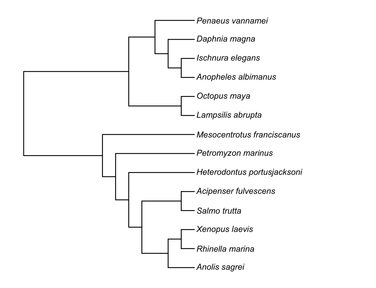

The 14-species tree returned by the one-call pipeline (pr_get_tree(source = "rotl", resolve_polytomies = TRUE, branch_lengths = "grafen")): ultrametric, fully bifurcating, with Grafen branch lengths. Tip labels are shown cleaned of the OTT id suffixes.

Confirm the two pipelines produce the same tree

# Same tip set?
setequal(res$tree$tip.label, res_manual$tree$tip.label)   # TRUE
# Same branch-length range (modulo RNG order for the bifurcation)?
range(res$tree$edge.length)
range(res_manual$tree$edge.length)
# Side-by-side plot
op <- par(mfrow = c(1, 2))
plot(res_manual$tree, main = "manual ape pipeline")
plot(res$tree,        main = "one-call pr_get_tree()")
par(op)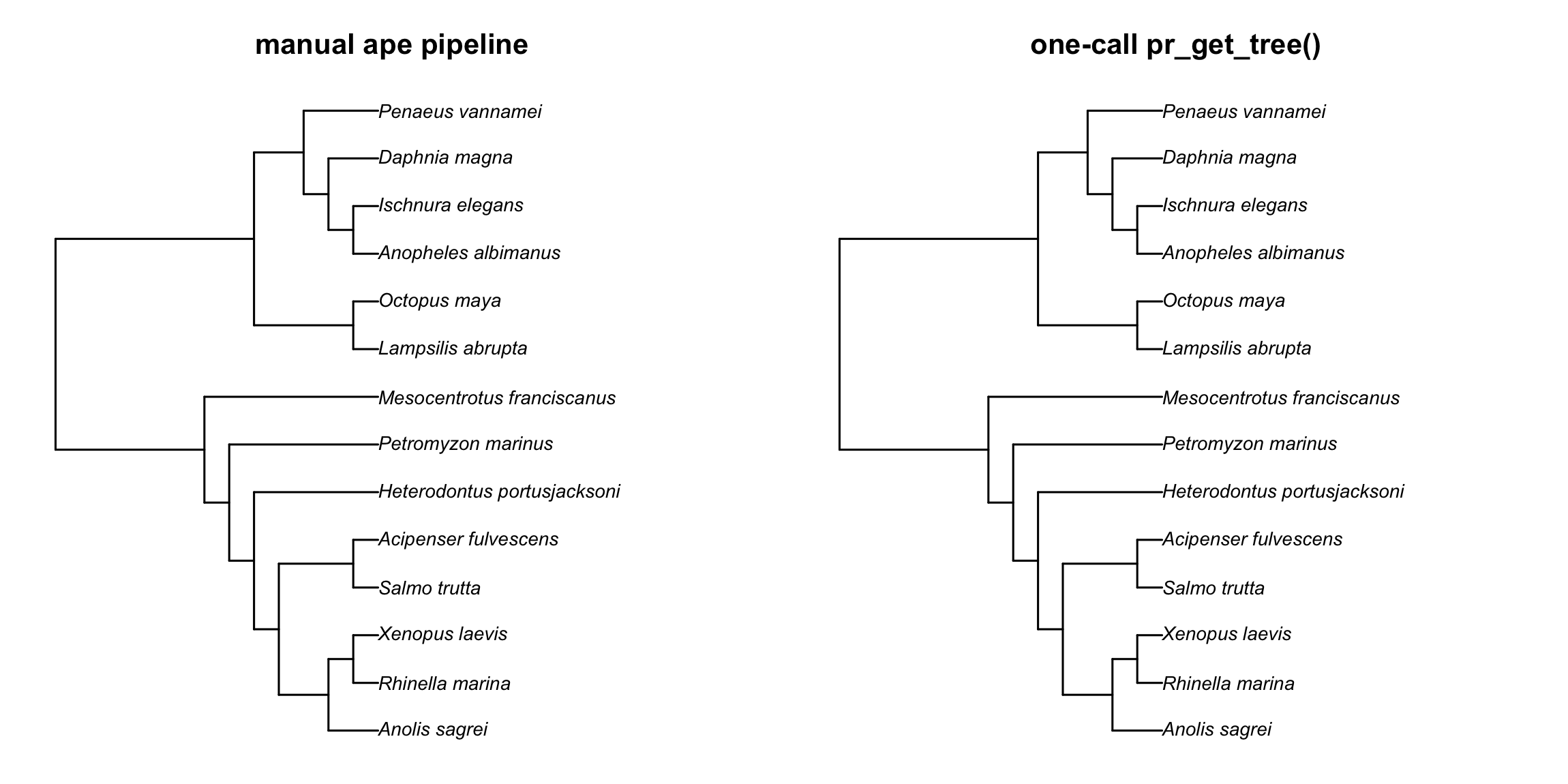

The manual ape pipeline (left) and the one-call pr_get_tree() (right) produce the same tree — same topology, same Grafen branch lengths.

About the _ott<digits> suffixes. Open Tree of Life identifies every taxon by an OTT id (e.g. Salmo_trutta_ott854188). rotl appends that id to the tip label so a downstream tool can verify which OTT node was placed. The suffix is informative for provenance but it makes the tip labels disagree with the binomial names you almost certainly have in your trait data frame ("Salmo trutta" vs "Salmo_trutta_ott854188"). The meta-analysis step below strips the suffix and converts underscores to spaces before computing the correlation matrix.

Step 4: phylogenetic correlation matrix

The tree currently has _ott<digits> suffixes and underscores in its tip labels. Strip those before computing the correlation matrix so the row / column names match the binomials in your trait data:

res$tree$tip.label <- gsub("_ott\\d+", "", res$tree$tip.label)
res$tree$tip.label <- gsub("_",        " ",  res$tree$tip.label)
res$tree$tip.label                          # now "Salmo trutta", etc.

Now compute the phylogenetic correlation matrix:

phy_cor <- pr_phylo_cor(res)
dim(phy_cor)            # 14 x 14 (one row/col per species)
isSymmetric(phy_cor)    # TRUE
all(diag(phy_cor) == 1) # TRUE (correlation matrix; ultrametric tree)
rownames(phy_cor)       # matches the binomials in `species`

pr_phylo_cor() is a thin wrapper around ape::vcv(tree, corr = TRUE). The function exists separately so the meta-analysis pattern is self-documenting and so the matrix can carry tree provenance.

Step 5: fit the meta-analysis with `metafor`

For the Pottier-style analysis, the effect size per study is the log response ratio (lnRR) of CTmax under contrasting developmental temperatures. Sampling variance comes with each effect via the group sample sizes / SDs. Suppose you’ve already extracted those per-study, per-species (this is the realistic shape of an ectotherm-thermal-tolerance dataset):

library(metafor)

# Toy effect-size data. Start by including every species at least
# once (otherwise random sampling can leave some species out and
# rma.mv complains about "levels in species without matching rows
# in R"). Then add 16 extra studies sampled with replacement to get
# a realistic multi-study-per-species shape.
set.seed(42)
toy_df <- data.frame(
  species = c(species,                          # 14 guaranteed rows
              sample(species, 16, replace = TRUE)),  # 16 extra
  study   = sprintf("study_%02d", seq_len(30)),
  yi      = rnorm(30, mean = 0.20, sd = 0.15),   # lnRR
  vi      = runif(30, min = 0.01, max = 0.08)    # sampling variance
)

# Sanity-check: every species in the data is also a row in phy_cor.
stopifnot(all(toy_df$species %in% rownames(phy_cor)))
length(intersect(toy_df$species, rownames(phy_cor)))   # 14

# Fit: random study effect (within-study) + random species effect
# (between-species, with phylogenetic correlation structure).
fit <- rma.mv(
  yi ~ 1,
  vi,
  random  = list(~1 | study, ~1 | species),
  R       = list(species = phy_cor),
  data    = toy_df,
  method  = "REML"
)
summary(fit)

A more robust alternative to the Step 4 label cleanup. The gsub() cleanup in Step 4 fixes label formatting, but it cannot catch species that are in your trait data yet absent from the tree (typos, synonyms, Open Tree of Life gaps). For those, align tree and data with reconcile_tree() + reconcile_apply() instead of the manual gsub(): this drops unresolved species and returns a data–tree pair guaranteed to match:

result <- reconcile_tree(
  x         = toy_df,
  tree      = res$tree,    # already gsub-cleaned, see Step 4
  x_species = "species",
  authority = NULL          # skip synonym lookup; tree labels already binomials
)
aligned <- reconcile_apply(
  result,
  data            = toy_df,
  tree            = res$tree,
  species_col     = "species",
  drop_unresolved = TRUE
)
phy_cor <- pr_phylo_cor(aligned$tree)
fit <- rma.mv(yi ~ 1, vi,
              random = list(~1 | study, ~1 | species),
              R      = list(species = phy_cor),
              data   = aligned$data,
              method = "REML")

The R = list(species = phy_cor) argument is what tells metafor that the species random effect has the correlation structure given by your phylogeny. The ~1 | study partitions within-study from between-species variance — standard for meta-analysis of multi-study effect-size data.

Pottier et al. used a slightly more complex metafor model including population, family, and shared-trial random effects (see their Statistical_analyses.Rmd). The phylogenetic component is the same R = list(species = phy_cor) either way.

Manual tree grafting when Open Tree of Life doesn’t have a species

A common situation: Open Tree of Life doesn’t have one of your species. Pottier et al. ran into this with Potamilus alatus (a freshwater mussel) — Open Tree of Life’s induced subtree errored on it, so they pulled it out of the TNRS match, generated the tree without it, then grafted it back manually with ape::bind.tip():

# Pottier et al.'s approach (paraphrased from their Rmd)

# Drop Potamilus alatus from the OTT id list: Open Tree of Life's
# induced-subtree service errors when this id is included.
taxa.tree <- filter(taxa, ott_id != "732215")

# Build the topology from the remaining OTT ids.
phylo_tree <- tol_induced_subtree(ott_ids = taxa.tree$ott_id)

# Resolve polytomies at random so the tree is strictly bifurcating
# (a full-rank phylogenetic correlation matrix needs this).
binary.tree <- multi2di(phylo_tree, random = TRUE)

# Graft Potamilus alatus back as a new tip at node 95 (inside
# Bivalvia). Attaching a tip *at* an existing node gives that node
# an extra child -- a polytomy -- which is why multi2di() ran first.
binary.tree <- bind.tip(binary.tree, tip.label = "Potamilus_alatus",
                        where = 95)

In prepR4pcm, the equivalent of “graft a species back in” is reconcile_augment(). Reconcile your trait data against the retrieved tree first; any species the tree does not carry lands in the reconciliation as unresolved. reconcile_augment() then grafts each unresolved species that has a congener already in the tree, and records the placement in $augmented for the methods section.

The worked example below adds Anolis carolinensis — a congener of Anolis sagrei, already in the 14-species tree from Steps 1-3 — and shows the species counts before and after grafting:

# Trait data carrying one species the retrieved tree lacks: Anolis
# carolinensis, a congener of Anolis sagrei (which is in the tree).
graft_df <- data.frame(
  species = c(res$tree$tip.label, "Anolis carolinensis")
)
nrow(graft_df)               # 15 species in the trait data

# Reconcile data names against the tree: 14 match, 1 is unresolved.
rec <- reconcile_tree(graft_df, res$tree,
                      x_species = "species", authority = NULL)

# Graft each unresolved species next to a congener already in the tree.
aug <- reconcile_augment(rec, res$tree)

aug$meta$original_n_tips     # 14  (tree tips before grafting)
aug$meta$augmented_n_tips    # 15  (tree tips after grafting)
aug$augmented[, c("species", "placed_near", "n_congeners")]
#>               species   placed_near n_congeners
#> 1 Anolis carolinensis Anolis sagrei           1

# The augmented tree is ready for a comparative model: still fully
# resolved, and still ultrametric.
ape::is.binary(aug$tree)       # TRUE
ape::is.ultrametric(aug$tree)  # TRUE

The trait data has 15 species; the retrieved tree had only 14 tips; after reconcile_augment() the tree carries all 15. Plotting the tree before and after makes the single added tip visible:

# reconcile_augment() writes the grafted tip label with an
# underscore; convert to a space for a consistent set of binomials.
aug$tree$tip.label <- gsub("_", " ", aug$tree$tip.label)

op <- par(mfrow = c(1, 2))
plot(aug$original, main = "Before grafting: 14 tips")
plot(aug$tree,     main = "After reconcile_augment(): 15 tips")
par(op)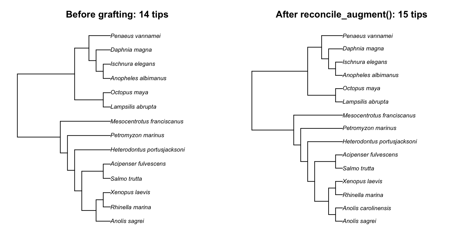

Left: the 14-tip Open Tree of Life topology before grafting. Right: the same tree after reconcile_augment() grafts Anolis carolinensis (15 tips). The new species joins as a bifurcating sister to its congener Anolis sagrei, and its terminal branch is adjusted so every tip stays aligned at the present: the augmented tree is bifurcating and ultrametric, ready for pr_phylo_cor().

Why the augmented tree has no polytomy. Manual bind.tip(where = 95) attaches the new tip at node 95, so that node gains a third child — a polytomy — which is why the Pottier pipeline runs multi2di() afterwards. reconcile_augment(), with its default where = "genus", instead inserts the new species part-way along the terminal branch of a congener: it splits that branch into a new two-way node, with the new species as one of the two children. The result is strictly bifurcating (ape::is.binary(aug$tree) returns TRUE), so no follow-up multi2di() is needed. Passing branch_length = "zero" or where = "near" attaches the tip at an existing node instead, and so produces a polytomy by design; see ?reconcile_augment.

The augmented tree also stays ultrametric. Phylogenetic comparative methods — pr_phylo_cor(), PGLS, phylogenetic meta-analysis — need an ultrametric tree: every species sits the same distance from the root, because all are extant and have had the same time to evolve. A grafted tip would not land exactly at the present on its own, so reconcile_augment() adjusts each grafted tip’s terminal branch afterwards to restore ultrametricity (ape::is.ultrametric(aug$tree) returns TRUE). The augmented tree therefore feeds straight into pr_phylo_cor() and a phylogenetic meta-analysis, exactly as in Steps 4-5.

The same one-species-manually-added pattern shows up in Cinar et al. (2022, Methods Ecol. Evol. 13:383), where Villosa delumbis was added based on ITIS — they describe it as “Polytomies were resolved at random, and one species, Villosa delumbis, was manually added to the tree based on information from the Integrated Taxonomic Information System.”

Why Grafen (and not DateLife / a time-calibrated tree)?

In principle you could replace Grafen branches with biologically real ones from DateLife:

# Alternative: get rotl topology, then date it with DateLife
res    <- pr_get_tree(species, source = "rotl",
                      resolve_polytomies = TRUE)   # NO branch_lengths
dated  <- pr_date_tree(res$tree)                   # DateLife dates it
phy_cor <- pr_phylo_cor(dated)

For most phylogenetic meta-analyses, we recommend Grafen, not DateLife, for three reasons:

Coverage. DateLife synthesises from per-clade published chronograms. For a cross-taxon dataset like Pottier’s (lampreys, bivalves, insects, fish, mammals etc., spanning 14 animal classes), DateLife usually can’t return a chronogram covering all of them — its database is sparse outside well-studied single-clade groups (mammals, birds, fish).
Question alignment. Phylogenetic meta-analysis models a species random effect with a phylogenetic correlation structure. The model asks “do related species have correlated effect sizes?”, not “how fast does the trait evolve per unit time?”. Pagel’s λ on the species random effect (which metafor estimates implicitly when you supply the correlation matrix) absorbs branch-length scale, so the choice between Grafen-units and time-units matters less than it would for, say, a Brownian-motion rate estimate.
Reproducibility. Grafen’s method is deterministic given the topology; DateLife results depend on which chronograms are in their database the day you run it.

Use DateLife instead when:

Your taxa fall within a single, well-studied clade (mammals, birds, insects-Lepidoptera, fish — see ?pr_date_tree).
The science question requires real divergence times (trait- evolution rate, Brownian-motion variance per million years, divergence-time questions).
You’re fitting a Brownian-motion-on-tree model directly (e.g. in caper::pgls or phylolm::phylolm) where branch-length scale enters the variance directly.

For the realistic cross-taxon meta-analysis case (the one Pottier et al. 2022 and many others run), Grafen via pr_get_tree(..., branch_lengths = "grafen") is the practical default.

What this vignette deliberately doesn’t cover

Mixed-effect specification. metafor::rma.mv() takes many more random/fixed structures than ~ 1 | species. See Viechtbauer
1. Journal of Statistical Software 36:1.
Branch-length sensitivity. The Cinar et al. simulation shows Grafen-vs-time-calibrated lengths matter. If your topology is time-calibrated (e.g. source = "fishtree" or source = "datelife"), don’t apply Grafen on top — pass branch_lengths = NULL (the default) and use the chronogram directly.
Multi-tree posterior. If your backend returns a multiPhylo, pr_phylo_cor() returns a list of correlation matrices. Feed each to metafor separately and pool with Rubin’s rules — see the posterior-tree pipeline vignette.