Effect decomposition

The picture no other SEM package draws

Every structural equation modelling tool will draw you a path diagram. None of them will draw you this: a forest plot that splits the total effect of a predictor into the part that travels through mediator means and the part that travels through mediator spread, zeros, or shape. That second channel – the distribution-mediated effect – is the reason drmSEM exists, and it is the figure below.

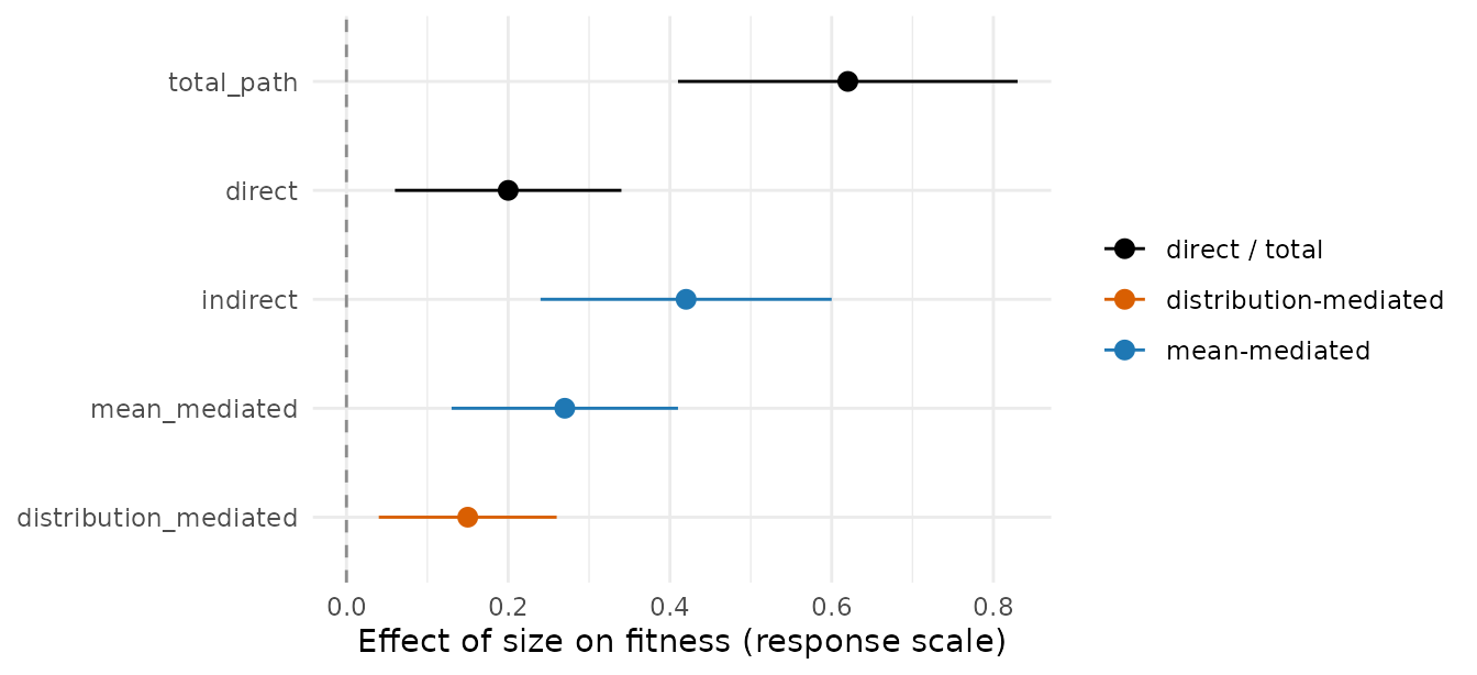
In this illustrative figure (the numbers above are hand-set, not estimated from data) the orange distribution_mediated interval sits clear of zero. That is the picture to look for: a part of how size reaches fitness flowing through the variability and zero-structure of an intermediate count rather than through any mean. A mean-only SEM reports that channel as zero, or silently folds it into the mean. drmSEM isolates it and labels it.

The three effect types

drmSEM distinguishes three ways a predictor X can reach a target node Y. The equations below (from docs/design/02-effect-calculus.md) name the exact component path each one travels.

• Direct. X -> mu(Y). The controlled direct effect (Robins and Greenland 1992; Pearl 2001): hold every mediator at its observed value and move only X, so just the arrows running directly into the mean of Y operate.

• Mean-mediated. X -> mu(M1) -> mu(M2) -> mu(Y). The classical indirect path: X shifts the mean of a mediator, which shifts the mean of the next, on down to the mean of Y.

• Distribution-mediated. X -> sigma(M2) -> distribution(M2) -> mu(Y). The part of the indirect effect that flows through a mediator’s scale (sigma), zero-inflation (zi), or shape (nu) rather than its mean. X changes how spread out (or how zero-inflated, or how skewed) the mediator is; that altered distribution, pushed through a curved downstream outcome, moves the mean of Y. Concretely it is a Jensen gap — the difference between propagating the mediator’s full distribution and propagating only its mean. It is therefore non-zero only when both a higher moment of the mediator responds to X and the outcome is nonlinear in that mediator: it is exactly zero under mean mediation, and zero when the outcome is linear in M even if sigma(M) depends on X.

That third type is what makes drmSEM distinctive: it has no coefficient-product analogue, because the signal lives in a distributional parameter and only becomes a mean effect after passing through a nonlinear link downstream — so a mean-only SEM reports it as zero. The estimand itself is not new: it is the interventional / distributional-mediation effect of the causal mediation literature (Pearl 2001; Imai et al. 2010; VanderWeele 2015, 2014; Vansteelandt and Daniel 2017). What is new is making a mediator’s sigma/zi/shape a first-class causal target in a piecewise distributional GLMM SEM and surfacing this term as a labelled, uncertainty-quantified row. It is identified under the usual mediation assumptions plus a correctly specified mediator distribution (its higher moments, not just its mean).

Why coefficient products are invalid here

The textbook mediation identity “indirect = product of path coefficients” is exact only on a single linear, identity-link scale. A drmSEM path routinely breaks both conditions:

• It crosses links. A log-link Poisson mean can feed a logit-link binomial mean downstream. Multiplying a coefficient defined on the log scale by one defined on the logit scale produces a number with no response-scale meaning.

• It crosses distributional components. A temp -> sigma(size) coefficient describes residual spread, not the mean. There is no valid arithmetic that multiplies a spread coefficient by a downstream mean coefficient to get a mean effect.

So drmSEM does not multiply coefficients. It simulates the intervention — the counterfactual / do-style propagation of Pearl (2009) and Imai et al. (2010): set the predictor to two contrasting values (a one-SD contrast for numerics, the first two levels for factors), push each contrast through the whole fitted DAG with random effects held at zero, and read off the conditional (RE = 0) response-scale change in the mean of the target. The distribution-mediated effect is only expressible at all under this simulation view – it has no coefficient-product counterpart to compare against.

The five-number decomposition

indirect_effects() returns five rows, one per quantity. Each is a contrast of simulated conditional (RE = 0) response-scale means between the high and low intervention.

quantity	meaning
total_path	the full simulated effect with mediators active and passing realized draws
direct	the controlled direct effect (mediators held inactive)
indirect	total_path - direct
mean_mediated	(mean-mediated total) - direct: the part carried by mediator means
distribution_mediated	(distribution total) - (mean total): the extra part flowing through mediator sigma / zi / nu

The identity to keep in mind is

indirect  ~=  mean_mediated  +  distribution_mediated

Reading the headline forest plot top to bottom: total_path is everything; direct is the slice that bypasses the mediators; indirect is what is left once the direct slice is removed; and that indirect slice splits into the blue mean_mediated part and the orange distribution_mediated part. When the orange interval excludes zero, you have evidence that the predictor acts on a mediator’s distribution shape, not just its location.

The canonical example: size -> abundance -> fitness

The data-generating process behind the headline figure (see the drmSEM introductory vignette and tests/testthat/helper-dgp.R for the full version) is an ecological chain where size reaches fitness through an intermediate count, abundance. Crucially, size is wired into a non-mean component of abundance: it inflates the spread / zero-structure of the count, not only its mean. That is what populates the distribution-mediated row.

The model is built and queried exactly as below. These chunks call the engine on a real fit, so they are shown but not run here.

# size      -> abundance (count): size acts on BOTH the NB mean and its
#              dispersion/zero-inflation, so it has a distributional channel.
# abundance -> fitness  (proportion alive out of trials).
sem <- drm_sem(
  abundance = drm_node(
    drmTMB::bf(abundance ~ size + temp, zi ~ size),   # size -> zi(abundance)
    family = drmTMB::nbinom2()
  ),
  fitness   = drm_node(
    drmTMB::bf(cbind(alive, dead) ~ abundance + size),
    family = drmTMB::beta_binomial()
  ),
  data = dat
)

paths() shows the component-labelled coefficients; note the size path into abundance appears once on mu and once on zi – two different claims.

paths(sem)

The controlled direct effect moves only size and lets nothing mediate:

direct_effects(sem, from = "size", to = "fitness")

The total effect under distribution mediation lets abundance pass realized draws from its negative-binomial family, so the spread and zeros it carries are included:

total_effects(sem, from = "size", to = "fitness", method = "simulate")

And the full five-number decomposition – the object plotted at the top of this vignette – comes from a single call:

eff <- indirect_effects(sem, from = "size", to = "fitness")
eff          # the five quantities as a table
plot(eff)    # the forest plot

plot() on the returned drm_effect draws the same forest plot rendered above: black for direct / total, blue for the mean-mediated channel, orange for the distribution-mediated channel, with a dashed reference line at zero.

Emphasis: the distribution-mediated channel

It is worth being explicit about what makes the orange row non-zero. In this example size enters zi(abundance) – the probability that a count is a structural zero. Larger organisms are found in patches that are present-or- absent more sharply, so size reshapes the zero-structure of abundance without (necessarily) moving its mean. When those realized, zero-heavy counts are pushed through the logit-link survival model, they move mean fitness. That movement is the distribution-mediated effect.

The same logic applies to any non-mean component:

• a path into sigma(M) – X makes a mediator more or less variable;
• a path into zi(M) or hu(M) – X changes the zeros or the hurdle;
• a path into nu(M) – X changes a shape parameter (tails / skew).

In each case the effect on Y is real provided the downstream outcome is curved in that mediator (a linear outcome has no Jensen gap, so the row is zero even when the mediator’s distribution responds to X); it is zero under mean mediation, and is reported on its own row, correctly labelled, by indirect_effects(). No other SEM package plots it as a separate row – which is exactly why this vignette opens with the figure that does.

Recap

• Three effect types: direct (X -> mu(Y)), mean-mediated (X -> mu(M) -> mu(Y)), and distribution-mediated (X -> sigma(M) -> distribution(M) -> mu(Y)).
• Effects are simulation-based, never coefficient products, because paths cross links and distributional components.
• indirect_effects() returns a five-number decomposition; the distribution_mediated row isolates the channel no coefficient-product method can express.
• plot() on the result is the marquee figure: a forest plot that makes the distributional channel visible.

For the full three-node worked system, d-separation, and Fisher’s C, see the drmSEM introductory vignette.

References

Imai, Kosuke, Luke Keele, and Teppei Yamamoto. 2010. “Identification, Inference and Sensitivity Analysis for Causal Mediation Effects.” Statistical Science 25 (1): 51–71. https://doi.org/10.1214/10-STS321.

Pearl, Judea. 2001. “Direct and Indirect Effects.” Proceedings of the Seventeenth Conference on Uncertainty in Artificial Intelligence (UAI), 411–20.

Pearl, Judea. 2009. Causality: Models, Reasoning, and Inference. 2nd ed. Cambridge University Press.

Robins, James M., and Sander Greenland. 1992. “Identifiability and Exchangeability for Direct and Indirect Effects.” Epidemiology 3 (2): 143–55. https://doi.org/10.1097/00001648-199203000-00013.

VanderWeele, Tyler J. 2014. “A Unification of Mediation and Interaction: A 4-Way Decomposition.” Epidemiology 25 (5): 749–61. https://doi.org/10.1097/EDE.0000000000000121.

VanderWeele, Tyler J. 2015. Explanation in Causal Inference: Methods for Mediation and Interaction. Oxford University Press.

Vansteelandt, Stijn, and Rhian M. Daniel. 2017. “Interventional Effects for Mediation Analysis with Multiple Mediators.” Epidemiology 28 (2): 258–65. https://doi.org/10.1097/EDE.0000000000000596.