Why a distributional piecewise SEM?
Most structural equation modelling treats a path
X -> Y as a statement about the expected
value of Y: increase X, and the mean
of Y shifts. That is only one of the things a predictor can
do. A predictor can also change how variable a response is, how
over-dispersed it is, how often it is a structural
zero, or how strongly two responses co-vary in their
residuals.
drmSEM makes those targets first-class — in the
distributional-regression tradition of Rigby and
Stasinopoulos (2005) and Brooks et al. (2017) — while keeping the
piecewise d-separation framework of Shipley (2009)
and Lefcheck (2016). It is the SEM / graph
/ d-separation / path / effect-decomposition layer; the drmTMB
package is the fitting engine. Each endogenous node is
exactly one drmTMB fit, the system is
piecewise, and the graph must be a
DAG. A causal path is
component-labelled: it targets one modelled
distributional component of a node:
| Component | Symbol | What a path to it means |
|---|---|---|
| mean | mu |
shifts the expected response |
| scale | sigma |
changes residual scale / dispersion, not the mean |
| shape | nu |
changes a shape parameter (e.g. tail/skew) |
| zero-infl. | zi |
changes the probability of a structural zero |
| hurdle | hu |
changes the probability of crossing the hurdle |
| RE scale | sd(group) |
changes among-group heterogeneity |
| residual r | rho12 |
changes the residual correlation between the two responses of a bivariate node |
The cardinal rule, enforced throughout the package: a path to
a non-mu component is never reported as a mean
effect. A temp -> sigma(size) path is a
statement about spread, and drmSEM keeps it
labelled as such everywhere – in paths(), in
plot(), and in the effect decomposition.
A rho12 target is the residual
correlation between two responses of a bivariate node
(eps_y1 <-> eps_y2); a path rho12 ~ x
says x changes that residual coupling – it is not
a mean effect and not a directed y1 -> y2
arrow. Targeting rho12 requires a bivariate
drmTMB fit (e.g.
family = c(gaussian(), gaussian()), with components
mu1/mu2/sigma1/sigma2/rho12)
supplied via drm_psem(); it is then extracted and labelled
like any other component path. The covariance-edge grammar now ships:
covary() declares a residual or higher-level covariance
edge, covariances() reports those edges separately from
paths(), and d-separation is aware of covarying responses
(dropping the y1 _||_ y2 claim). The bivariate-node
declaration grammar now also ships: drm_pair() declares a
joint two-response node, rho12() / corpairs()
report the declared edges, and plot() draws them as
double-headed (residual) / dashed (higher-level) arcs.
drm_sem() fits one joint bivariate drmTMB
model for a drm_pair(); rho12() reads the
coefficients back (see
docs/design/07-bivariate-covariance-edges.md).
A worked system:
size -> abundance -> survival
The biological question. Body size,
local abundance, and survival form a causal
chain, and temperature (temp) is the exogenous driver. We
want to answer one question end to end: does warming reach survival
only by shifting the average size and abundance, or also by
changing how variable size is and how often abundance collapses
to a structural zero? The second half of that question is about
non-mean components (sigma, zi), which a
mean-only SEM cannot represent. By the end of this vignette we will read
the answer directly off the distribution_mediated row of
indirect_effects().
We use a three-node ecological chain. Conceptually:
-
sizeof organisms depends on temperature and habitat. We also let temperature act on the scale of size:sigma(size) ~ temp. Equation:size ~ Normal(mu = b0 + b1*temp + b2*habitat, sigma = exp(g0 + g1*temp)). -
abundanceis a count depending onsizeandtemp, modelled with a negative binomial, with habitat acting on zero-inflation:zi(abundance) ~ habitat. Equation (link scale):log(mu) = a0 + a1*size + a2*temp,logit(zi) = c0 + c1*habitat. -
survivalis a binomial proportion (cbind(alive, dead)) depending onabundanceandsize, with a beta-binomial family to absorb extra-binomial variation:logit(mu) = d0 + d1*abundance + d2*size.
Temperature is exogenous and reaches survival only
indirectly – through the mean, the scale, and the
zero-inflation of the intermediate nodes. That is exactly the
situation where coefficient-product mediation breaks down and a
distribution-aware, simulation-based decomposition is required.
Simulate the data
# This chunk uses only base R, so it always runs.
set.seed(1)
n <- 400L
habitat <- factor(sample(c("A", "B"), n, replace = TRUE))
temp <- rnorm(n)

# size: mean depends on temp + habitat; SCALE (sigma) depends on temp.
mu_size <- 2 + 0.8 * temp + 0.5 * (habitat == "B")
sd_size <- exp(-0.2 + 0.4 * temp)            # temp -> sigma(size)
size <- rnorm(n, mu_size, sd_size)

# abundance: NB mean depends on size + temp; ZI depends on habitat.
mu_ab <- exp(0.5 + 0.3 * size + 0.2 * temp)
zi_ab <- plogis(-1 + 1.2 * (habitat == "B"))  # habitat -> zi(abundance)
abundance <- ifelse(rbinom(n, 1, zi_ab) == 1, 0,
                    rnbinom(n, mu = mu_ab, size = 2))

# survival: binomial proportion out of a fixed number of trials.
trials <- 20L
p_surv <- plogis(-1 + 0.05 * abundance + 0.15 * size)
alive <- rbinom(n, trials, p_surv)
dead <- trials - alive

dat <- data.frame(temp, habitat, size, abundance, alive, dead)
head(dat)
#>         temp habitat      size abundance alive dead
#> 1  0.4094018       A 1.9985932         0     6   14
#> 2  1.6888733       B 6.2683461        28    15    5
#> 3  1.5865884       A 4.0851891         0     3   17
#> 4 -0.3309078       A 2.1241479         3     8   12
#> 5 -2.2852355       B 0.6269537         0     7   13
#> 6  2.4976616       A 1.4706468         9     8   12
The data-generating process puts a real signal into a
non-mean component of two different nodes
(sigma(size) and zi(abundance)), which is what
we want the SEM to recover and propagate.
Build the SEM
drm_sem() takes one named drm_node() per
endogenous response and a shared data frame. Each
drm_node() wraps a drmTMB::bf() formula (which
can carry component sub-formulas like sigma ~ temp or
zi ~ habitat) and a family.
sem <- drm_sem(
  size      = drm_node(drmTMB::bf(size ~ temp + habitat, sigma ~ temp),
                       family = stats::gaussian()),
  abundance = drm_node(drmTMB::bf(abundance ~ size + temp, zi ~ habitat),
                       family = drmTMB::nbinom2()),
  survival  = drm_node(drmTMB::bf(cbind(alive, dead) ~ abundance + size),
                       family = drmTMB::beta_binomial()),
  data = dat
)
#> ℹ Fitting node "size"
#> ✔ Fitting node "abundance" [116ms]
#>
#> ℹ Fitting node "abundance"
#> ✔ Fitting node "survival" [130ms]
#>
#> ℹ Fitting node "survival"
#> ✔ Fitting node "survival" [108ms]
#>
If you have already fitted nodes yourself, drm_psem()
assembles a SEM from existing drmTMB objects instead of
fitting internally; both routes produce the same object.
Inspect the component-labelled paths
paths() returns one row per fitted fixed-effect
coefficient across all nodes, each tagged with the
component it targets and the link on
which it acts. This is where the distributional structure becomes
legible: the temp path into size appears twice
– once on mu, once on sigma – and they are not
the same claim.
paths(sem)
#> <drmSEM paths: 8 component-labelled coefficients>
#>       from        to component     link      term estimate std.error statistic
#>       temp      size        mu identity      temp   0.7981    0.0335    23.816
#>    habitat      size        mu identity  habitatB   0.4803    0.0705     6.817
#>       temp      size     sigma      log      temp   0.4544    0.0366    12.406
#>       size abundance        mu      log      size   0.3210    0.0523     6.140
#>       temp abundance        mu      log      temp   0.2288    0.0728     3.142
#>    habitat abundance        zi    logit  habitatB   1.3045    0.2555     5.105
#>  abundance  survival        mu    logit abundance   0.0484    0.0059     8.245
#>       size  survival        mu    logit      size   0.1627    0.0198     8.206
#>    p.value endogenous
#>  2.25e-125      FALSE
#>   9.27e-12      FALSE
#>   2.42e-35      FALSE
#>   8.28e-10       TRUE
#>   1.68e-03      FALSE
#>   3.31e-07      FALSE
#>   1.65e-16       TRUE
#>   2.29e-16       TRUE
Each row is one fitted fixed-effect coefficient, with columns
from, to, component,
link, term, estimate,
std.error, statistic, p.value,
and endogenous. The component column is what
makes the table distributional: the same predictor can appear against
mu, sigma, zi, and so on, and
each is a different scientific claim. The structure looks like this
(column shape is real; the numbers are illustrative, not estimated):
#>        from        to component     link      term
#> 1      temp      size        mu identity      temp
#> 2   habitat      size        mu identity  habitatB
#> 3      temp      size     sigma      log      temp
#> 4      size abundance        mu      log      size
#> 5      temp abundance        mu      log      temp
#> 6   habitat abundance        zi    logit  habitatB
#> 7 abundance  survival        mu    logit abundance
#> 8      size  survival        mu    logit      size
Note how temp -> size appears twice – once on
mu (does warming shift mean size?) and once on
sigma (does warming change how variable size is?)
– and habitat -> abundance lands on zi, the
probability of a structural zero, not on the mean count. These are the
rows a mean-only SEM cannot express.
check_sem() reports, per node, the family, the modelled
components, convergence, whether a fixed-effect covariance is available
(needed for d-separation and effect intervals), and whether a
realized-value sampler exists (needed for fully distribution-mediated
effects).
check_sem(sem)
#>
#> ── drmSEM diagnostics ──
#>
#>       node        family components nobs converged vcov_available sampler
#>       size      gaussian  mu, sigma  400      TRUE           TRUE    TRUE
#>  abundance       nbinom2     mu, zi  400      TRUE           TRUE    TRUE
#>   survival beta_binomial         mu  400      TRUE           TRUE    TRUE
#> Exogenous variables: "temp" and "habitat"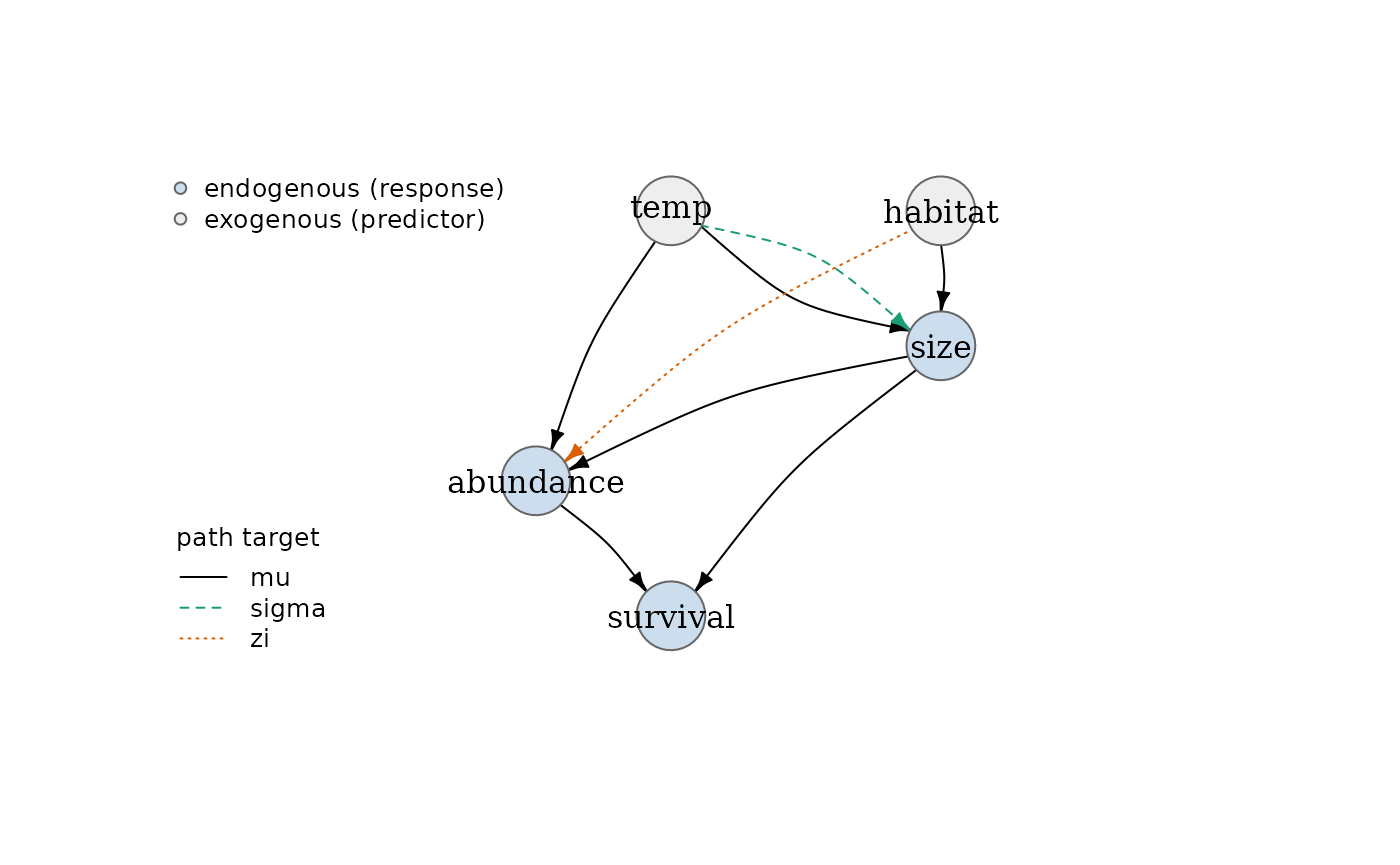
d-separation and Fisher’s C
A piecewise SEM is tested by checking the independence
claims the DAG implies (Pearl 2009; Shipley
2000, 2009): every pair of
non-adjacent nodes should be conditionally independent given their
parents. basis_set() lists those claims.
basis_set(sem)
#>                                       claim       x        y           given
#> 1    temp _||_ survival | {abundance, size}    temp survival abundance, size
#> 2 habitat _||_ survival | {abundance, size} habitat survival abundance, size
In drmSEM, d-separation uses the any-component
LRT. A missing arrow X -> Y asserts that
X has no effect on any modelled component
of Y. We test it by refitting Y’s node
augmented with X in each component sub-model and comparing
to the baseline by a likelihood-ratio test:
LRT = 2 * (logLik(augmented) - logLik(baseline)),
distributed (asymptotically) as chi-squared with degrees of freedom
equal to the number of added coefficients across components.
dsep() runs this for every claim in the basis set.
dsep(sem)
#> <drmSEM d-separation: 2 claims>
#>                                      claim       x        y           given df
#>     temp _||_ survival | {abundance, size}    temp survival abundance, size  1
#>  habitat _||_ survival | {abundance, size} habitat survival abundance, size  1
#>     LR p.value status n_effective scale_group
#>  2.500   0.114     ok          NA        <NA>
#>  1.003   0.317     ok          NA        <NA>
#> Fisher's C = 6.65 on 4 df, p = 0.156
fisher_c() combines the per-claim p-values into Fisher’s
C statistic, C = -2 * sum(log(p_i)), with 2k
degrees of freedom for k claims. A small p-value flags a
missing path – including a missing path into a non-mean
component, which a mean-only SEM tool could never detect.
fisher_c(sem)
#>   fisher_c df n_claims   p.value n_extreme n_excluded
#> 1 6.646451  4        2 0.1557935         0          0
Decomposing effects by simulation
Coefficient products are not a valid way to combine paths
across non-Gaussian links or across distributional components.
drmSEM therefore computes effects by Monte-Carlo
propagation over the fitted DAG — the counterfactual,
do()-style framework of Pearl (2001), Pearl (2009) and Imai
et al. (2010): it sets the exogenous
predictor to two contrasting values, pushes the change through every
downstream node, and reads the conditional (RE = 0)
response-scale change in the mean of the target.
Direct (controlled) effect. Hold all mediators at
their observed values; move only temp. Only the arrows that
go directly into survival operate.
direct_effects(sem, from = "temp", to = "survival")
#> <drmSEM effect>
#>  from       to    scale target estimate conf.low conf.high
#>  temp survival response   mean        0        0         0
Total effect. Let every mediator respond. With
method = "simulate", mediators pass realized draws
from their fitted families, so effects flowing through a mediator’s
sigma, zi, or nu are included.
With method = "gcomp" (the default), only mediator means
propagate.
total_effects(sem, from = "temp", to = "survival", method = "simulate")
#> <drmSEM effect>
#>  from       to    scale    mediation target estimate conf.low conf.high
#>  temp survival response distribution   mean   0.8985   0.7278    1.0868
Indirect effect with a distributional decomposition.
This is the heart of the package. indirect_effects()
reports five quantities:
-
total_path– the full simulated effect through the chosen mediators; -
direct– the controlled direct effect; -
indirect–total_path - direct; -
mean_mediated– the part carried by mediator means; -
distribution_mediated– the extra effect that appears only when mediators pass realized draws, i.e. the part flowing through scale, zero-inflation, or shape (total under distributionminustotal under mean).
indirect_effects(sem, from = "temp", to = "survival")
#> <drmSEM effect>
#>  from       to         through target              quantity estimate conf.low
#>  temp survival size, abundance   mean            total_path   0.9015   0.7488
#>  temp survival size, abundance   mean                direct   0.0000   0.0000
#>  temp survival size, abundance   mean              indirect   0.9015   0.7488
#>  temp survival size, abundance   mean         mean_mediated   0.8537   0.7085
#>  temp survival size, abundance   mean distribution_mediated   0.0478   0.0223
#>  conf.high
#>     1.0794
#>     0.0000
#>     1.0794
#>     1.0306
#>     0.0787
The result is one row per quantity, each an effect on
the response (probability-of-survival) scale, with an estimate and a
confidence interval. The shape – and how to read it – looks like this
(illustrative numbers, not estimated here):
#>   from       to              quantity estimate conf.low conf.high
#> 1 temp survival            total_path    0.090    0.052     0.128
#> 2 temp survival                direct    0.020    0.004     0.036
#> 3 temp survival              indirect    0.070    0.038     0.102
#> 4 temp survival         mean_mediated    0.048    0.022     0.074
#> 5 temp survival distribution_mediated    0.022    0.006     0.038
Read it top-down. total_path is the whole effect of
warming on survival; direct is the slice that does
not go through the mediators; indirect is the rest
(total_path - direct). The indirect slice then
splits into mean_mediated (carried by the means of
size and abundance) and distribution_mediated – and
indirect ≈ mean_mediated + distribution_mediated.
That last row is the answer to the question we posed at the start. A
non-trivial distribution_mediated row is the signature of
this framework: temperature reaches survival partly because it changes
the spread of size and (via habitat structure) the
zeros of abundance, not only their means. A mean-only SEM would
report that channel as zero or silently fold it into the mean.
drmSEM keeps it visible and correctly labelled.
(plot() on an effect object draws the same decomposition as
a forest plot.)
Standardizing
When you need comparable path strengths, standardize()
returns the paths() table with one added column,
std.estimate (on the link scale), while preserving the
component labels. The default method = "sd_x" scales each
coefficient by the standard deviation of its predictor;
method = "latent" additionally divides by the fitted
standard deviation of the response, giving fully standardized
coefficients.
standardize(sem)                      # adds std.estimate (sd_x scaling)
#> <drmSEM standardized paths (sd_x, 1sd): 8 component-labelled coefficients>
#>       from        to component     link      term estimate std.error statistic
#>       temp      size        mu identity      temp   0.7981    0.0335    23.816
#>    habitat      size        mu identity  habitatB   0.4803    0.0705     6.817
#>       temp      size     sigma      log      temp   0.4544    0.0366    12.406
#>       size abundance        mu      log      size   0.3210    0.0523     6.140
#>       temp abundance        mu      log      temp   0.2288    0.0728     3.142
#>    habitat abundance        zi    logit  habitatB   1.3045    0.2555     5.105
#>  abundance  survival        mu    logit abundance   0.0484    0.0059     8.245
#>       size  survival        mu    logit      size   0.1627    0.0198     8.206
#>    p.value endogenous std.estimate
#>  2.25e-125      FALSE       0.8303
#>   9.27e-12      FALSE       0.4803
#>   2.42e-35      FALSE       0.4727
#>   8.28e-10       TRUE       0.4379
#>   1.68e-03      FALSE       0.2380
#>   3.31e-07      FALSE       1.3045
#>   1.65e-16       TRUE       0.2639
#>   2.29e-16       TRUE       0.2220
standardize(sem, method = "latent")   # fully standardized
#> <drmSEM standardized paths (latent, 1sd): 8 component-labelled coefficients>
#>       from        to component     link      term estimate std.error statistic
#>       temp      size        mu identity      temp   0.7981    0.0335    23.816
#>    habitat      size        mu identity  habitatB   0.4803    0.0705     6.817
#>       temp      size     sigma      log      temp   0.4544    0.0366    12.406
#>       size abundance        mu      log      size   0.3210    0.0523     6.140
#>       temp abundance        mu      log      temp   0.2288    0.0728     3.142
#>    habitat abundance        zi    logit  habitatB   1.3045    0.2555     5.105
#>  abundance  survival        mu    logit abundance   0.0484    0.0059     8.245
#>       size  survival        mu    logit      size   0.1627    0.0198     8.206
#>    p.value endogenous std.estimate
#>  2.25e-125      FALSE       0.9752
#>   9.27e-12      FALSE       0.5641
#>   2.42e-35      FALSE       1.0000
#>   8.28e-10       TRUE       0.5804
#>   1.68e-03      FALSE       0.3155
#>   3.31e-07      FALSE       1.9975
#>   1.65e-16       TRUE       0.1419
#>   2.29e-16       TRUE       0.1194
Recap
-
drmSEMis a layer on thedrmTMBengine; onedrmTMBfit per endogenous node, DAG-only, observed variables only. - Paths are component-labelled (
mu,sigma,nu,zi,hu,sd(group),rho12); a non-mupath is never a mean effect. - d-separation is the any-component LRT, combined by Fisher’s C.
- Direct / indirect / total effects are simulation-based, never coefficient products, and the indirect decomposition exposes distribution-mediated pathways explicitly.
For the environment and CI setup that compiles and installs the
drmTMB engine, see CLOUD.md; for the operating
contract, see AGENTS.md.