Calibrating the d-separation test

This page answers one practical question: when dsep() says the graph does not need a missing arrow, how often is that conclusion wrong? All results are precomputed on live drmTMB; this document performs no model fitting. The study object is regenerated only in the drmTMB lane and ships as a cached .rds inside the package.

Bottom line

The calibration grid checks whether drmSEM’s d-separation test (Shipley 2000, 2009) keeps its false-positive rate near the nominal level under a correct graph, and whether it rejects a graph when an omitted edge is truly present. The simulation study follows the design principles of Morris et al. (2019). In this cached run, all five acceptance checks passed.

• Type-I error across the null cells ranged from 0.025 to 0.080 at nominal alpha 0.05.
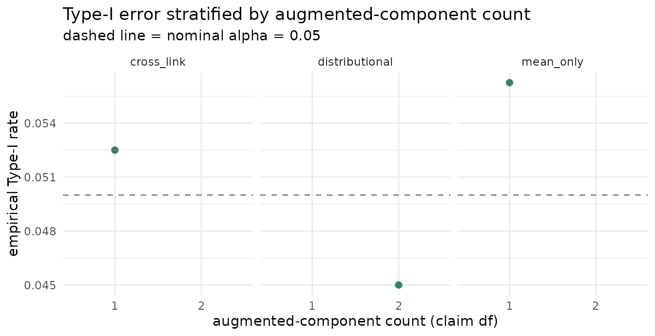
• Type-I error stayed inside its Monte-Carlo band when grouped by the number of response components augmented during the test: 1 component: 0.052; 2 components: 0.045; 1 component: 0.056.
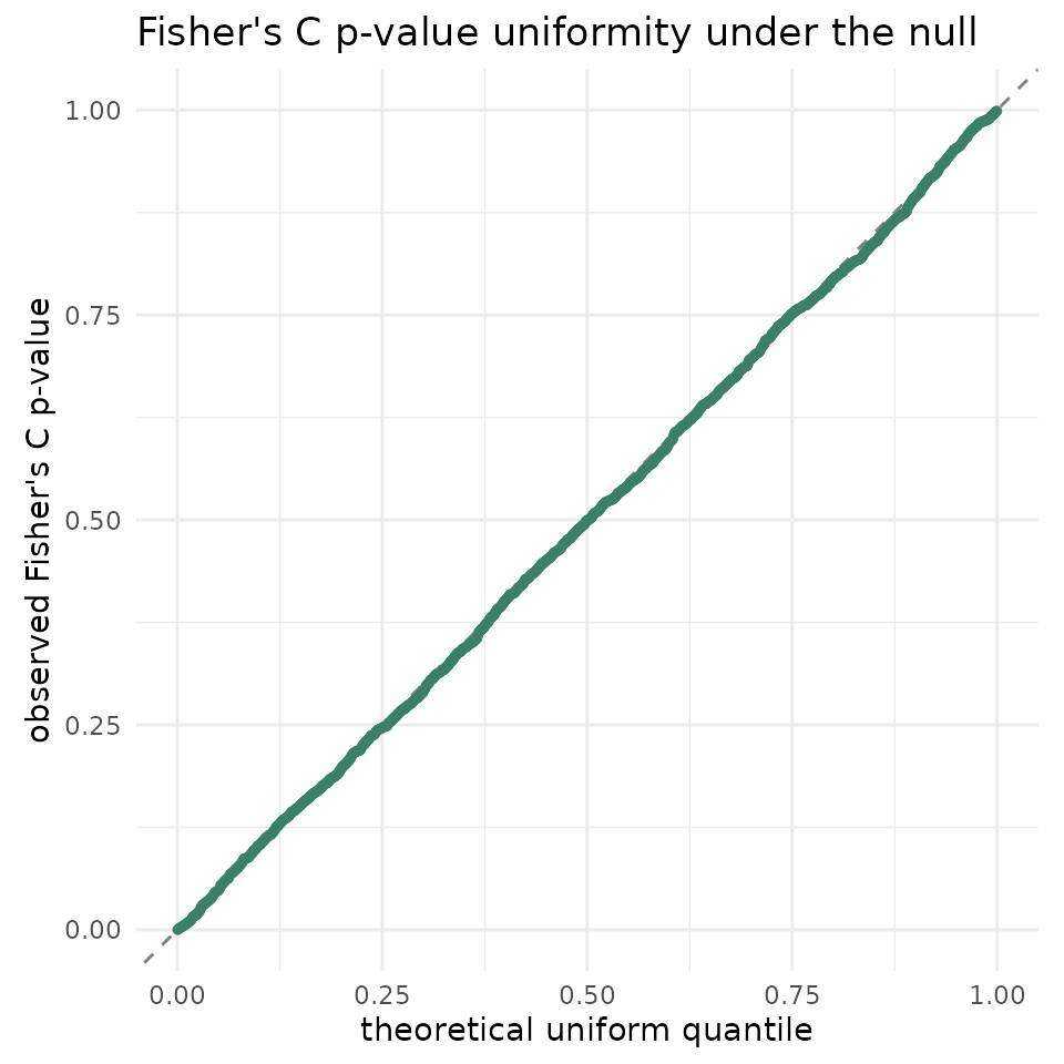
• Fisher’s C p-values under the null were close to Uniform(0, 1): KS p = 0.631, median p = 0.499.
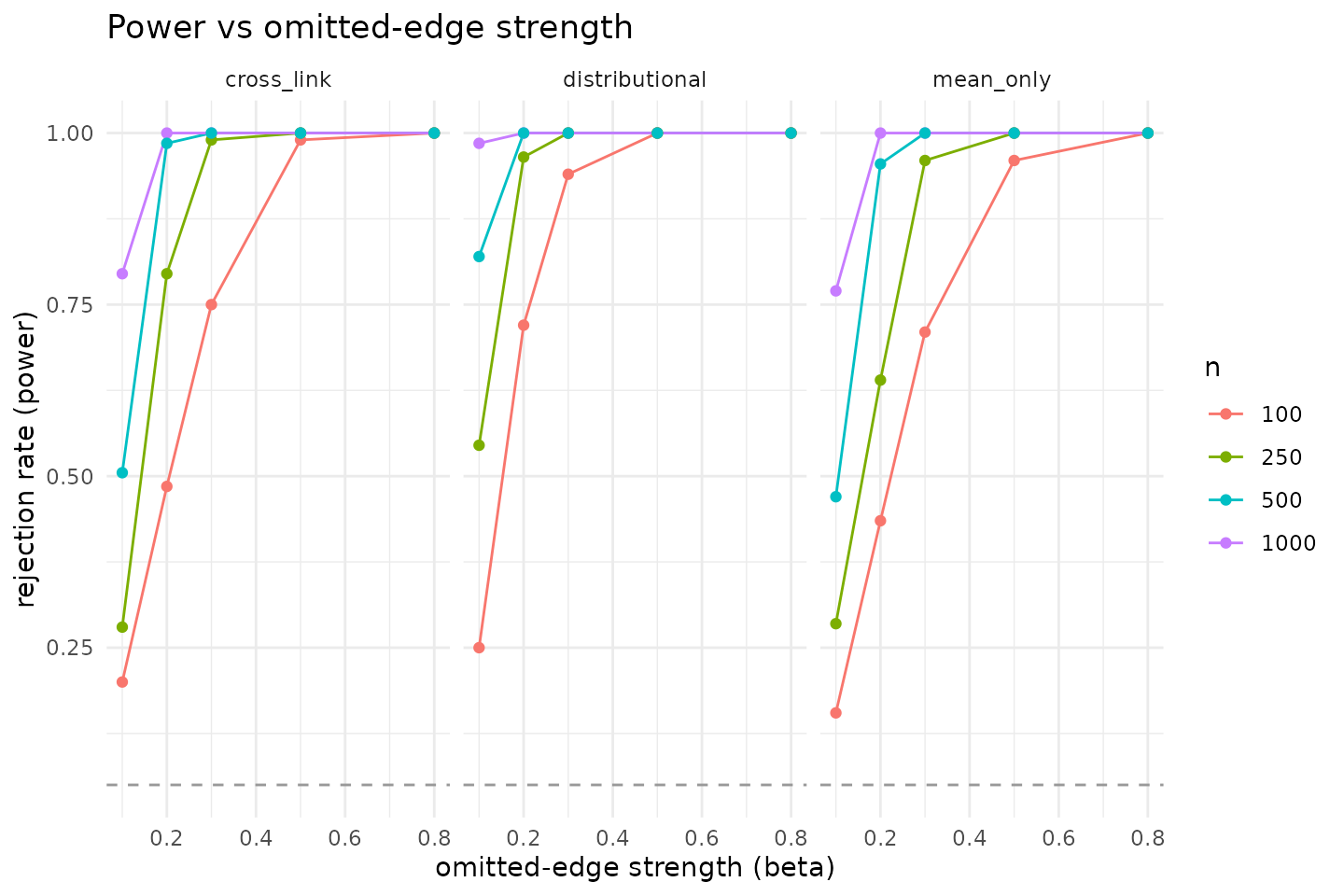
• Power at the moderate omitted-edge strength beta = 0.5 was at least 1.00 for n >= 250; power at beta = 0.8 was 1.00 in every tested cell.

The claim is deliberately scoped: this validates the tested grid below. It does not prove that every possible distributional SEM, every random-effect structure, or every future drmTMB family is calibrated.

What is being tested

In a piecewise SEM, each missing arrow is a statistical claim: after conditioning on the right variables, the two nodes should be independent. dsep() turns that claim into a likelihood-ratio test. Because drmSEM models whole conditional distributions, not just means, the test adds the candidate predictor to every modelled component of the response node: mu, sigma, zi, and so on. That is the any-component d-separation rule.

Calibration asks whether this test behaves like its nominal p-value says it should. Under a correct graph, a 5% test should reject about 5% of the time (Type-I error). When the graph omits a real edge, the rejection rate should rise as the omitted effect gets stronger (power). Fisher’s C then combines the individual d-separation p-values into one graph-level check.

The important stress point is the number of response components augmented in a claim. A mean-only response adds one extra parameter; a response with both mu and sigma modelled adds two. If the any-component rule were miscalibrated, the problem would likely show up as this augmented-component count increases.

It is deliberately distinct from the fast smoke check in tests/testthat/test-calibration.R, which runs only 20 reps of a single chain to catch gross regressions in CI. That smoke test is not calibration evidence; this cached study is.

Study design

The grid sweeps four sample sizes, six omitted-edge strengths, and three data-generating-process (DGP) families, with many replicates per cell.

GRID <- list(
  n      = c(100, 250, 500, 1000),
  beta   = c(0, 0.1, 0.2, 0.3, 0.5, 0.8),   # strength of the OMITTED x -> y edge
  family = c("mean_only", "distributional", "cross_link"),
  reps   = 200
)

Each DGP is a chain x -> m -> y whose true graph also contains a direct x -> y edge of strength beta. We fit the SEM without that edge. The basis-set claim x _||_ y | {m} is therefore true exactly when beta == 0 (Type-I error) and false when beta > 0 (power). The three DGP families differ in which distributional component the omitted edge enters:

# mean-only: omitted edge perturbs the MEAN of y
y <- rnorm(n, beta * x + 0.7 * m, 1)

# distributional: omitted edge perturbs the SPREAD (sigma) of y, not its mean
y <- rnorm(n, 0.7 * m, exp(beta * x))   # could equally drive zi for a count y

# cross-link: m is distributionally driven by x (its sigma), omitted edge on
# the mean of y -- exercises an augmented refit over a multi-component node
m <- rnorm(n, 0.5 * x, exp(0.3 * x))
y <- rnorm(n, beta * x + 0.7 * m, 1)

# For each cell and replicate: build the SEM, run dsep(), and record the
# x _||_ y | {m} claim's p-value, its df (= number of augmented components),
# its status, and the per-replicate Fisher's C p-value. (Schematic; the
# authoritative version is inst/calibration/generate.R.)
sem <- drm_sem(
  m = drm_node(drmTMB::bf(m ~ x), family = gaussian()),
  y = drm_node(drmTMB::bf(y ~ m), family = gaussian()),
  data = dat
)
d  <- dsep(sem)
p  <- d$p.value[d$x == "x" & d$y == "y"]
df <- d$df[d$x == "x" & d$y == "y"]          # augmented-component count
fc <- attr(d, "fisher_c")$p.value

This study code is shown for transparency only and is never evaluated when the vignette is built.

Acceptance criteria

The cached study object stores these checks in cal$acceptance. We treat the calibration claim on this page as passing only if all five checks pass:

1. Every family x n x beta cell has at least 95% usable d-separation claims (status == "ok" and finite p-value).
2. Every beta = 0 family x n Type-I estimate lies inside the 99% binomial Monte-Carlo band around the nominal alpha.
3. Every beta = 0 family x augmented-component-count (claim_df) Type-I estimate lies inside the same 99% Monte-Carlo band.
4. Fisher’s C p-values under the null are close to Uniform(0, 1): one-sample KS p >= 0.01 and median p in [0.40, 0.60].
5. Power behaves as expected: beta = 0.8 gives power >= 0.80 in every family x n cell; beta = 0.5 gives power >= 0.70 for n >= 250; and power is nondecreasing aside from at most 0.05 Monte-Carlo jitter.

Acceptance checks for the d-separation calibration grid.

Criterion	Rule	Pass
usable claim rate	Every family x n x beta cell has at least 95% ok finite claim p-values.	TRUE
Type-I by family and n	Every beta=0 family x n cell lies inside the 99% binomial Monte-Carlo band around alpha.	TRUE
Type-I by augmented-component count	Every beta=0 family x claim_df stratum lies inside the 99% binomial Monte-Carlo band around alpha.	TRUE
Fisher’s C null uniformity	Null Fisher’s C p-values have KS p >= 0.01 and median in [0.40, 0.60].	TRUE
power against omitted edges	At beta=0.8 every family x n cell has power >= 0.80; at beta=0.5 and n>=250 power >= 0.70; power is nondecreasing up to 0.05 Monte-Carlo jitter.	TRUE

Type-I error by family and sample size

Empirical Type-I rate at nominal alpha = 0.05, with the 99% Monte-Carlo acceptance band.

	DGP family	n	Type-I	MC lower	MC upper	reps	pass
1	cross_link	100	0.075	0.015	0.095	200	TRUE
3	cross_link	250	0.030	0.015	0.095	200	TRUE
4	cross_link	500	0.025	0.015	0.095	200	TRUE
2	cross_link	1000	0.080	0.015	0.095	200	TRUE
5	distributional	100	0.045	0.015	0.095	200	TRUE
7	distributional	250	0.035	0.015	0.095	200	TRUE
8	distributional	500	0.070	0.015	0.095	200	TRUE
6	distributional	1000	0.030	0.015	0.095	200	TRUE
9	mean_only	100	0.080	0.015	0.095	200	TRUE
11	mean_only	250	0.035	0.015	0.095	200	TRUE
12	mean_only	500	0.050	0.015	0.095	200	TRUE
10	mean_only	1000	0.060	0.015	0.095	200	TRUE

The centerpiece: Type-I stratified by augmented-component count

The any-component refit adds the candidate predictor to every modelled component of the response, so the claim’s degrees of freedom equal the number of augmented components. Mis-calibration, if it exists, is most likely to show up as the component count grows – which is exactly what this figure isolates.

Fisher’s C uniformity under the null

Under a correctly specified DAG (beta == 0), the per-replicate Fisher’s C p-value should be Uniform(0, 1). Departures from the diagonal in the QQ plot flag mis-calibration of the combined test.

Power curves

Rejection rate against the omitted-edge strength beta, faceted by sample size and DGP family. A well-behaved test climbs from the nominal level at beta = 0 toward 1 as the omitted edge strengthens.

How this was generated

The cache backing this page is built by inst/calibration/generate.R, run in the live-drmTMB lane:

Rscript inst/calibration/generate.R

That script guards on requireNamespace("drmTMB"), sweeps the full grid above, collects only data (per-claim p-values, df, status, and per-replicate Fisher’s C p-values – never fitted objects), and writes a compact summary list to inst/calibration/calibration-results.rds. The cache carries a meta stamp recording the drmTMB version, date, R version, and git SHA so every figure on this page is traceable to the exact engine that produced it.

#> Cache provenance:
#>   generated:      2026-06-06 19:27:54 UTC
#>   drmTMB version: 0.1.3.9000
#>   drmTMB SHA:     17b132119eeef40ac6a9655a7372281844007ae6
#>   drmSEM version: 0.2.0.9000
#>   R version:      R version 4.5.2 (2025-10-31)
#>   git SHA:        c951d31
#>   reps per cell:  200

References

Morris, Tim P., Ian R. White, and Michael J. Crowther. 2019. “Using Simulation Studies to Evaluate Statistical Methods.” Statistics in Medicine 38 (11): 2074–102. https://doi.org/10.1002/sim.8086.

Shipley, Bill. 2000. “A New Inferential Test for Path Models Based on Directed Acyclic Graphs.” Structural Equation Modeling 7 (2): 206–18. https://doi.org/10.1207/S15328007SEM0702_4.

Shipley, Bill. 2009. “Confirmatory Path Analysis in a Generalized Multilevel Context.” Ecology 90 (2): 363–68. https://doi.org/10.1890/08-1034.1.