
library(pigauto)
data(avonet300, tree300)
set.seed(42)
tree <- ape::keep.tip(tree300, sample(tree300$tip.label, 80))
traits <- avonet300[match(tree$tip.label, avonet300$Species_Key),
                    c("Mass", "Wing.Length", "Trophic.Level",
                      "Primary.Lifestyle"), drop = FALSE]
rownames(traits) <- tree$tip.label
traits$Mass[1:8] <- NA
traits$Wing.Length[6:13] <- NA
traits$Trophic.Level[4:11] <- NA
traits$Primary.Lifestyle[10:17] <- NA
x <- preprocess_traits(traits, tree)
Imagine assembling a comparative dataset of bird body mass, wing length, trophic level and lifestyle. The first two are continuous measurements; the last two are categorical traits. Here we use 80 birds from the bundled AVONET data and deliberately remove some entries to make the example reproducible. The gaps are assigned by position in the tree’s tip order, so they can cluster among relatives. They illustrate the plots; they do not reproduce a known real-world missingness process. Start with the missingness plots to decide whether the available measurements are distributed across the tree or concentrated in particular groups.
Before fitting, compare missing fractions and inspect the observation-by-trait matrix. Labels include trait types; each expanded categorical trait is represented once.
plot_missingness(x, "summary")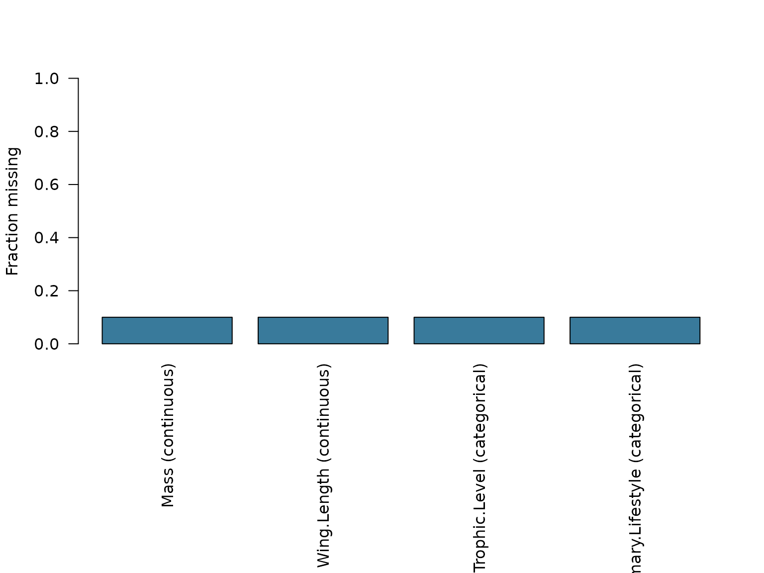
plot_missingness(x, "matrix")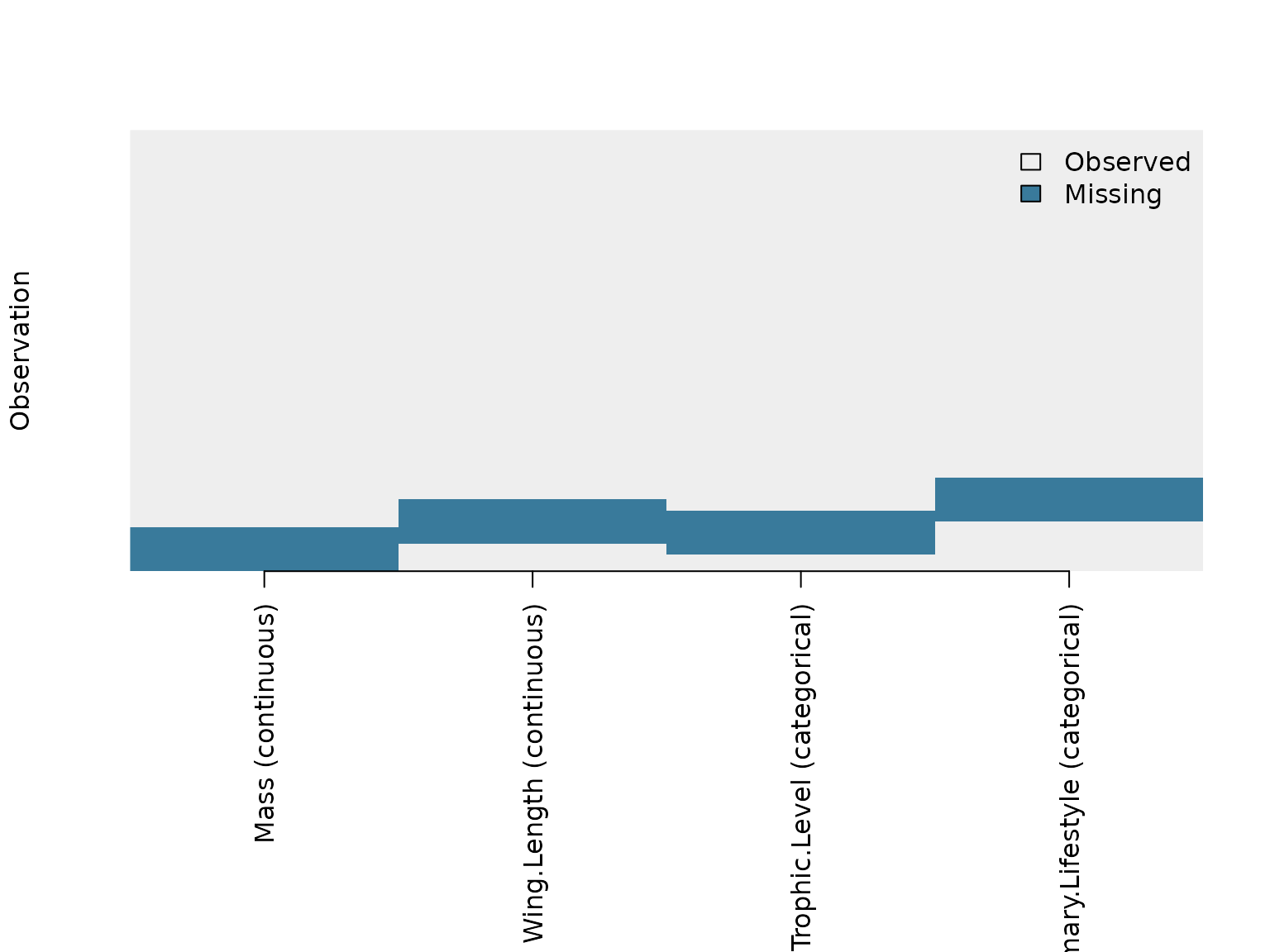
The tree-ordered matrix places related tips close together, helping reveal clades with more missing data. The co-missingness map reports the fraction of all observations missing each pair of traits, including the marginal fraction on its diagonal. Such patterns guide investigation; neither plot establishes the missingness mechanism or proves data are missing completely at random.
plot_missingness(x, "phylo", tree)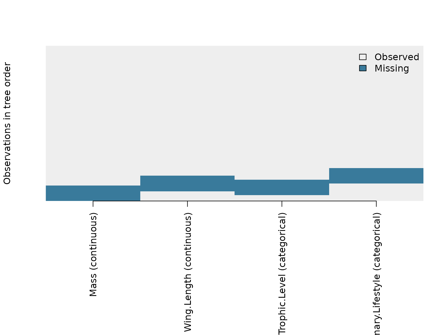
plot_missingness(x, "co_missing")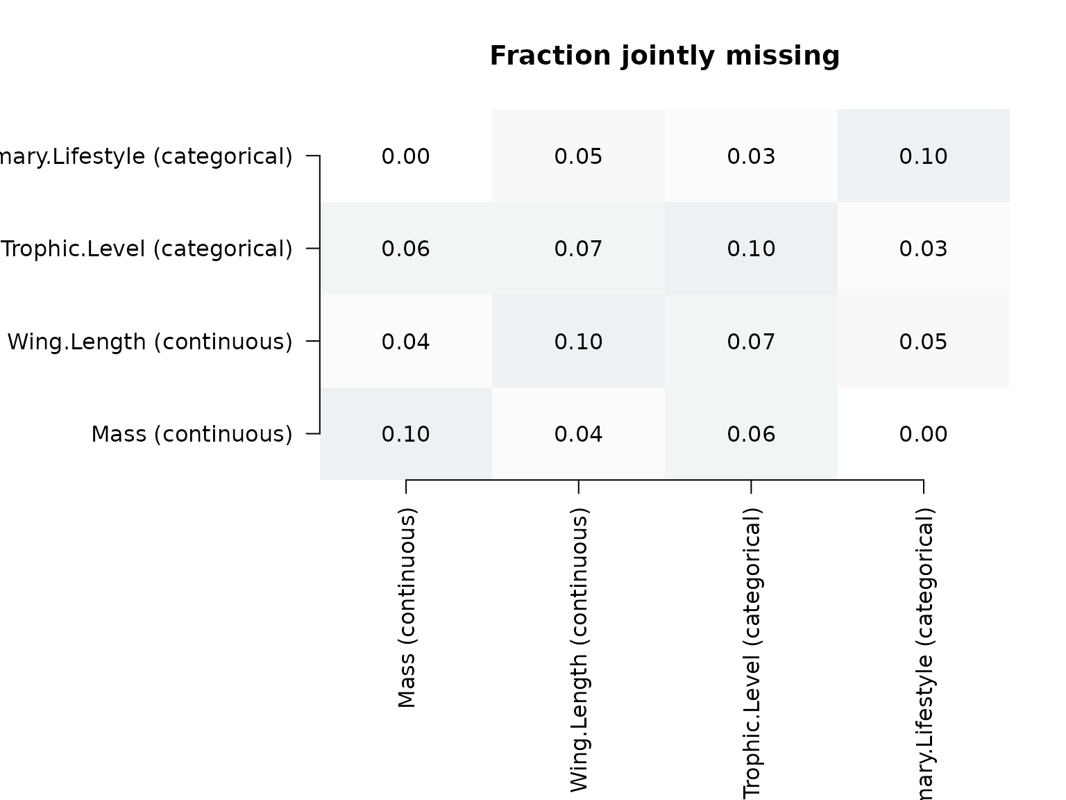
Inspecting individual predictions
Fit the mixed traits together, then inspect the predicted mass and its conformal bounds for a few birds whose mass we removed. The bounds are on the original mass scale, so they can be read alongside the prediction. They give an exploratory sense of the range of plausible values for an individual missing measurement, which can help decide which values need closer scrutiny. The same dataset also contains categorical traits, but these numeric conformal bounds are not categorical confidence intervals. Here the true mass is known because we removed it ourselves; in a real application it would need to be measured independently to check an individual prediction.
result <- impute(traits, tree, gnn = FALSE, verbose = FALSE, seed = 7)## Warning: Small validation set for 4 trait(s): Mass (n=6), Wing.Length (n=9),
## Trophic.Level (n=11), Primary.Lifestyle (n=10). Calibrated gate and conformal
## scores will be noisy for these trait(s). 95% split-conformal coverage is NOT
## achievable for 2 trait(s) with fewer than 19 validation cells (Mass (n=6),
## Wing.Length (n=9)): the achievable ceiling is n_val / (n_val + 1), which only
## reaches 0.95 at n_val >= 19. See `?fit_pigauto` under 'Calibration at small n'
## for smoothing options.
missing_mass <- which(is.na(traits$Mass))
mass_predictions <- data.frame(
  species = rownames(traits)[missing_mass],
  predicted_mass_g = result$prediction$imputed[missing_mass, "Mass"],
  lower_g = result$prediction$conformal_lower[missing_mass, "Mass"],
  upper_g = result$prediction$conformal_upper[missing_mass, "Mass"],
  hidden_mass_g = avonet300$Mass[match(rownames(traits)[missing_mass],
                                       avonet300$Species_Key)],
  row.names = NULL
)
mass_predictions
## species predicted_mass_g lower_g upper_g hidden_mass_g
## 1 Rhea_americana 1529.05331 442.31031 5285.8909 23000.0
## 2 Ptilopachus_petrosus 54.45561 15.75241 188.2514 193.0
## 3 Bambusicola_fytchii 81.56036 23.59302 281.9517 313.7
## 4 Tympanuchus_phasianellus 163.41141 47.27013 564.9083 882.4
## 5 Dendrocygna_guttata 173.56145 50.20624 599.9967 800.0
## 6 Rhynochetos_jubatus 180.04049 52.08044 622.3945 860.0
## 7 Lampornis_clemenciae 139.26004 40.28385 481.4177 7.6
## 8 Hylocharis_chrysura 139.26004 40.28385 481.4177 4.5Plot just the missing masses, using a log scale because bird masses span a wide range. The dot is the point prediction, the line its exploratory conformal interval, and the cross the measurement we deliberately hid. In an actual dataset the cross would be unavailable for a genuinely missing value. An especially broad interval, or a hidden value outside its interval, prompts closer investigation rather than unquestioning reliance on the imputation.
ggplot2::ggplot(mass_predictions,
  ggplot2::aes(x = predicted_mass_g, y = species,
               xmin = lower_g, xmax = upper_g)) +
  ggplot2::geom_pointrange(orientation = "y") +
  ggplot2::geom_point(ggplot2::aes(x = hidden_mass_g),
                      shape = 4, colour = "#B33A3A", size = 2.5) +
  ggplot2::scale_x_log10() +
  ggplot2::labs(x = "Predicted body mass (g; log scale)", y = NULL,
                title = "Missing body masses: predictions and exploratory intervals") +
  ggplot2::theme_minimal()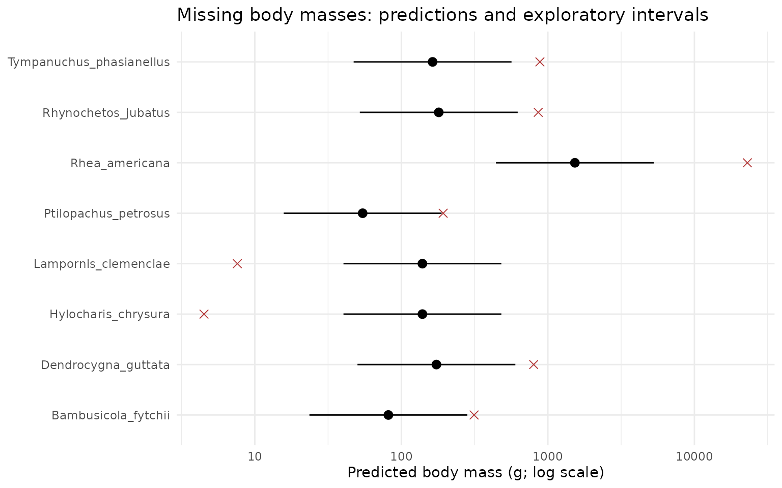
In this particular example, none of the eight hidden masses falls inside its interval. The greater rhea’s hidden mass is 23,000 g, while its predicted mass is about 1,529 g. The eight were chosen by tree position and include very large and very small birds: the rhea is larger than every remaining observed bird, and one hummingbird is smaller than all of them. Their prediction errors are large relative to the calibration errors. These eight selected gaps are not an independent random sample, so their 0/8 coverage is not an estimate of general performance. The red crosses are possible here only because we started with recorded values and hid them ourselves.
The fit also warns that only six mass observations were available to calibrate the interval score. That is too few to support the usual finite-sample 95% split-conformal guarantee with a finite empirical bound, even before considering whether the calibration and missing species are exchangeable. We show the warning deliberately: inspect it when interpreting your own fit.
These are prediction intervals for missing trait values, not confidence intervals for a regression coefficient. Their nominal 95% coverage is not certified for this dataset. Standard conformal coverage depends on calibration and future cases being exchangeable; related species, clade-structured missingness and differences between observed and missing species can make that assumption questionable. A small calibration set also makes the bounds unstable, and wide bounds can cover values while offering little practical precision. Examine held-out coverage and interval width, using the number of test values and species- or clade-level holdouts relevant to your question. The single fit above does not establish 95% coverage.
For a categorical trait, inspect the predicted class separately. Here are the birds with an artificially missing trophic level. These labels are point predictions; a numeric mass interval does not quantify their class uncertainty.
missing_diet <- which(is.na(traits$Trophic.Level))
data.frame(
  species = rownames(traits)[missing_diet],
  predicted_trophic_level = result$prediction$imputed[missing_diet, "Trophic.Level"],
  hidden_trophic_level = avonet300$Trophic.Level[
    match(rownames(traits)[missing_diet], avonet300$Species_Key)],
  row.names = NULL
)
## species predicted_trophic_level hidden_trophic_level
## 1 Tympanuchus_phasianellus Herbivore Herbivore
## 2 Dendrocygna_guttata Herbivore Omnivore
## 3 Rhynochetos_jubatus Carnivore Carnivore
## 4 Lampornis_clemenciae Carnivore Herbivore
## 5 Hylocharis_chrysura Carnivore Herbivore
## 6 Tachymarptis_melba Carnivore Carnivore
## 7 Telacanthura_ussheri Carnivore Carnivore
## 8 Geotrygon_linearis Herbivore HerbivoreThe hidden labels let us see individual mistakes in this demonstration. In practice, use a separate held-out evaluation to assess accuracy and compare it with a simple baseline; do not read these eight examples as a performance study.
Conformal scores are quantiles of held-out errors on an encoded trait scale; they help construct bounds but do not measure prediction accuracy or establish coverage on their own. Conformal-based multiple-imputation draws are for prediction diagnostics, not Rubin pooling. For downstream estimates and confidence intervals, use a supported analysis-aware or posterior multiple- imputation route, and check its documented scope and validation limitations. Eligibility for pooling does not itself establish reliable inference for your analysis; see the validation results.
Checking prediction accuracy
Use held-out observed values to assess point predictions. For example:
evaluate(result$fit)## method trait type metric value
## 1 pigauto Mass continuous rmse 0.6013815
## 2 pigauto Mass continuous pearson_r 0.9728627
## 3 pigauto Mass continuous mae 0.4897527
## 4 pigauto Mass continuous conformal_coverage_95 0.8461538
## 5 pigauto Wing.Length continuous rmse 0.2880914
## 6 pigauto Wing.Length continuous pearson_r 0.9465866
## 7 pigauto Wing.Length continuous mae 0.2573158
## 8 pigauto Wing.Length continuous conformal_coverage_95 1.0000000
## 9 pigauto Trophic.Level categorical accuracy 0.5000000
## 10 pigauto Trophic.Level categorical accuracy_Carnivore 1.0000000
## 11 pigauto Trophic.Level categorical accuracy_Herbivore 0.0000000
## 12 pigauto Trophic.Level categorical accuracy_Omnivore 0.0000000
## 13 pigauto Primary.Lifestyle categorical accuracy 0.7500000
## 14 pigauto Primary.Lifestyle categorical accuracy_Aerial 0.0000000
## 15 pigauto Primary.Lifestyle categorical accuracy_Insessorial 1.0000000
## 16 pigauto Primary.Lifestyle categorical accuracy_Terrestrial 0.0000000
## 17 baseline Mass continuous rmse 0.6013815
## 18 baseline Mass continuous pearson_r 0.9728627
## 19 baseline Mass continuous mae 0.4897527
## 20 baseline Wing.Length continuous rmse 0.2880914
## 21 baseline Wing.Length continuous pearson_r 0.9465866
## 22 baseline Wing.Length continuous mae 0.2573158
## 23 baseline Trophic.Level categorical accuracy 0.5000000
## 24 baseline Trophic.Level categorical accuracy_Carnivore 1.0000000
## 25 baseline Trophic.Level categorical accuracy_Herbivore 0.0000000
## 26 baseline Trophic.Level categorical accuracy_Omnivore 0.0000000
## 27 baseline Primary.Lifestyle categorical accuracy 0.7500000
## 28 baseline Primary.Lifestyle categorical accuracy_Aerial 0.0000000
## 29 baseline Primary.Lifestyle categorical accuracy_Insessorial 1.0000000
## 30 baseline Primary.Lifestyle categorical accuracy_Terrestrial 0.0000000
## n_test
## 1 13
## 2 13
## 3 13
## 4 13
## 5 9
## 6 9
## 7 9
## 8 9
## 9 6
## 10 3
## 11 2
## 12 1
## 13 8
## 14 1
## 15 6
## 16 1
## 17 13
## 18 13
## 19 13
## 20 9
## 21 9
## 22 9
## 23 6
## 24 3
## 25 2
## 26 1
## 27 8
## 28 1
## 29 6
## 30 1Reading the prediction metrics
The test values are observations that pigauto deliberately hid before
fitting. Their true values remain available for checking predictions.
They are different from the genuinely missing values, whose prediction
errors we cannot measure without collecting new observations. Use
evaluate(result$fit) for this check. If you need a
prediction object for lower-level scoring, request
predict(result$fit, evaluation = TRUE); production
predictions may use the observed values you would otherwise be treating
as hidden.
| Metric | Meaning | How to read it |
|---|---|---|
| RMSE on the standardized latent scale (zRMSE) | Square root of the average squared difference between predictions and hidden values, after the trait’s transformation and standardization. | Smaller is better; zero means exact agreement on these cells. A value of 0.5 is half a preprocessing standard deviation on this scale, not half an original measurement unit. Squaring gives larger errors more weight. |
| Accuracy for binary or categorical traits | Fraction of hidden class labels predicted correctly. | Larger is better; 0.8 means 80% correct. Compare with the majority-class prediction: 80% accuracy is uninformative if predicting the commonest class already achieves 90%. |
| Correlation | How predictions and hidden values vary together. | High correlation does not rule out a systematic shift or an incorrect prediction scale. Inspect error measures too. |
| Conformal score | A high quantile of absolute validation errors, used to set prediction-bound width for supported traits. | It is measured on the encoded trait scale. A larger value gives wider bounds; it does not by itself demonstrate that those bounds cover missing values at the nominal rate. |
| Held-out coverage | Fraction of hidden test values inside the reported bounds. | Read it with the number of test values and interval width. A small test set gives an imprecise coverage estimate; broad bounds can cover many values without being useful. |
For continuous, count, ordinal and proportion traits,
evaluate() reports RMSE on the encoded scale. Depending on
the trait, that scale uses log, log1p, integer ranks or logit before
standardization. The HTML report labels this “RMSE (latent scale)”. The
standardization makes units explicit but provides no universal good/bad
threshold: compare predictions on the same hidden cells with a suitable
simple reference and consider the biological cost of an error. Other
metrics, such as zero-inflated-count RMSE and compositional errors, have
their own scales; see ?evaluate_imputation.
A point prediction and an individual completed-data draw answer
different questions. Score the point prediction to assess its error. To
assess a predictive distribution, consider coverage together with width
or a suitable distributional score. Scoring each stochastic completion
adds its draw variation to prediction error; that alone does not
establish whether the uncertainty is appropriate.
mi$pooled_point is the selected route’s point completion,
not generally an average of the returned m datasets.