Building up: from lm to location-scale • symbolizer

The idea

New to symbolizer? Skim vignette("symbolizer") first — a five-minute quickstart on a single model. This article is the next step up: it climbs from lm to a location-scale model so you can watch the symbolic story grow.

symbolizer turns any fitted model into a structured symbolic specification. To see what that buys you, the easiest path is to fit a sequence of models — each adding one feature — and watch the symbolic specification grow rung by rung.

Throughout this article we use one dataset — body mass measured across temperature, sex, and site — and climb four rungs:

Rung	Model	What’s new in the symbolic story
1	`lm(body_mass ~ temperature)`	distribution + linear predictor
2	`lm(body_mass ~ temperature + sex)`	a factor: dummy-encoded contrast
3	lmer(body_mass ~ temperature + sex + (1 \| site))	a random intercept + variance components
4	drmTMB(body_mass ~ temperature + sex + (1 \| site), sigma ~ temperature)	heteroscedasticity: variance depends on temperature

The reader-facing surface stays exactly the same: at every rung you call symbolize(fit), then as_latex() / symbol_table() / parameter_interpretation() to read it. The contents of those outputs grow.

Setup — one shared dataset

library(symbolizer)
set.seed(1)

n <- 200
n_sites <- 12
sites <- factor(rep(paste0("S", sprintf("%02d", seq_len(n_sites))),
                    length.out = n))
site_effect <- rnorm(n_sites, 0, 1.5)[as.integer(sites)]
sex <- factor(sample(c("F", "M"), n, replace = TRUE))
temperature <- runif(n, 10, 25)

# Mean: linear in temperature, +0.7 for males, plus a site offset.
# Variance: heteroscedastic — residual SD grows with temperature.
mu_true    <- 30 + 0.4 * temperature + 0.7 * (sex == "M") + site_effect
sigma_true <- exp(0.3 + 0.05 * temperature)
body_mass  <- rnorm(n, mean = mu_true, sd = sigma_true)

dat <- data.frame(
  body_mass   = body_mass,
  temperature = temperature,
  sex         = sex,
  site        = sites
)
head(dat, 4)
#>   body_mass temperature sex site
#> 1  36.82290    23.85953   F  S01
#> 2  32.86767    17.66440   F  S02
#> 3  37.65935    13.86432   M  S03
#> 4  40.17388    10.69691   F  S04

The “truth” the ladder will gradually uncover:

Slope of temperature on the mean: 0.4 g per °C
Sex contrast (M − F) on the mean: +0.7 g
Site-to-site SD on the mean: 1.5 g
Heteroscedasticity: residual SD grows by a factor of exp(0.05) ≈ 1.05 per °C

Rung 1 — A linear model

The simplest fit. Just temperature on the mean.

fit1 <- lm(body_mass ~ temperature, data = dat)
sym1 <- symbolize(fit1)

The equation:

equations(sym1, notation = "index")

\begin{aligned} \mathrm{body\_mass}_i \mid \mu_i,\, \sigma \sim \mathrm{Normal}(\mu_i,\, \sigma^2) \\ \mu_i = \beta_{0} + \beta_{1} \, \mathrm{temperature}_i \end{aligned}

The symbol dictionary, listing every variable the model uses:

symbol_table(sym1)

index	matrix	variable	units	role	shape	concrete	description
\mathrm{body\_mass}_i	\mathbf{body\_mass}	body_mass	NA	response	\mathbb{R}^n	\mathbb{R}^{200}	response variable
\mathrm{temperature}_i	—	temperature	NA	predictor	column of design matrix	column of X (length 200)	continuous predictor
\mu_i	\boldsymbol{\mu}	NA	NA	parameter	\mathbb{R}^n	\mathbb{R}^{200}	conditional mu of body_mass
\sigma	\boldsymbol{\sigma}	NA	NA	residual_sd	scalar (constant across observations)	scalar	residual standard deviation of body_mass
\beta_{0}, \beta_{1}	\boldsymbol{\beta}	NA	NA	coefficient	\mathbb{R}^{p_\mu}	\mathbb{R}^{2}	mu submodel coefficients
—	\mathbf{X}	NA	NA	design_matrix	\mathbb{R}^{n \times p_\mu}	\mathbb{R}^{200 \times 2}	mu submodel design matrix

What each coefficient means, on each scale symbolizer knows about:

parameter_interpretation(sym1, scale = "biological")

submodel	term_label	coefficient_role	estimate	95% CI	biological_reading
mu	(Intercept)	intercept	32.4	30.4, 34.4 *	Baseline body_mass in the reference condition
mu	temperature	slope	0.303	0.190, 0.415 *	A unit change in temperature shifts the expected body_mass by 0.303

Rows marked * have a 95% confidence interval that excludes zero (CI method: wald).

What we have so far. A distribution line for the response, a linear predictor for \mu_i, and one slope to interpret. No variance modelling beyond a single residual SD. No grouping. The biological reading is “a unit change in temperature shifts the expected body_mass by 0.303.”

Rung 2 — Adding a factor

What if mass differs systematically between sexes? Add sex to the mean.

fit2 <- lm(body_mass ~ temperature + sex, data = dat)
sym2 <- symbolize(fit2)

equations(sym2, notation = "index")

\begin{aligned} \mathrm{body\_mass}_i \mid \mu_i,\, \sigma \sim \mathrm{Normal}(\mu_i,\, \sigma^2) \\ \mu_i = \beta_{0} + \beta_{1} \, \mathrm{temperature}_i + \beta_{2} \, [sex = \mathrm{M}] \end{aligned}

The equation now carries a contrast term. The symbol dictionary adds a row for the dummy-encoded contrast:

symbol_table(sym2)

index	matrix	variable	units	role	shape	concrete	description
\mathrm{body\_mass}_i	\mathbf{body\_mass}	body_mass	NA	response	\mathbb{R}^n	\mathbb{R}^{200}	response variable
\mathrm{temperature}_i	—	temperature	NA	predictor	column of design matrix	column of X (length 200)	continuous predictor
\mathrm{sex}_i	—	sex	NA	factor	column of design matrix	column of X (length 200)	factor (F [reference], M)
\mu_i	\boldsymbol{\mu}	NA	NA	parameter	\mathbb{R}^n	\mathbb{R}^{200}	conditional mu of body_mass
\sigma	\boldsymbol{\sigma}	NA	NA	residual_sd	scalar (constant across observations)	scalar	residual standard deviation of body_mass
\beta_{0}, \beta_{1}, \beta_{2}	\boldsymbol{\beta}	NA	NA	coefficient	\mathbb{R}^{p_\mu}	\mathbb{R}^{3}	mu submodel coefficients
—	\mathbf{X}	NA	NA	design_matrix	\mathbb{R}^{n \times p_\mu}	\mathbb{R}^{200 \times 3}	mu submodel design matrix

sex is a factor with reference level F (alphabetical). The single dummy column [sex = M] enters the linear predictor with its own slope \beta_2. The interpretation reads the contrast explicitly:

pi2 <- parameter_interpretation(sym2, scale = "biological")
pi2[pi2$coefficient_role == "factor_contrast", c("term_label", "estimate", "biological_reading")]

term_label	estimate	biological_reading
sex	0.410	Average body_mass differs between M and F by 0.410

What just got added. One row in the symbol table (the factor contrast), one row in parameter_interpretation(), and one term in the LaTeX. The model class didn’t change (lm to lm), but the symbolic story grew exactly where the model grew.

Rung 3 — Adding random effects

Sites probably differ from one another, even at the same temperature. Add a random intercept per site.

library(lme4)
#> Loading required package: Matrix
#> 
#> Attaching package: 'Matrix'
#> The following object is masked from 'package:symbolizer':
#> 
#>     expand
fit3 <- lmer(body_mass ~ temperature + sex + (1 | site), data = dat)
sym3 <- symbolize(fit3)

equations(sym3, notation = "index")

\begin{aligned} \mathrm{body\_mass}_i \mid \mu_i,\, \sigma \sim \mathrm{Normal}(\mu_i,\, \sigma^2) \\ \mu_i = \beta_{0} + \beta_{1} \, \mathrm{temperature}_i + \beta_{2} \, [sex = \mathrm{M}] + u_{site(i)} \\ u_{site} \sim \mathcal{N}(0,\, \sigma_{site}^2) \end{aligned}

Two new rows in the equation block:

u_{site(i)} is added to the linear predictor for \mu_i.
A second distributional line: u_{site} ~ N(0, σ²_site).

Variance components are now first-class:

sym3$variance_components

parameter	group	term	sd_estimate	var_estimate
mu	site	(Intercept)	1.17	1.36
residual	residual	Residual	3.29	10.8

You can read off the between-site SD and the residual SD directly. The fixed-effect interpretation rows for temperature and sex still read on the response scale; what changed is that the model now partitions the variability into between-site and within-site parts.

What just got added. A u_{site(i)} symbol, a random-effect distributional line, and a variance_components tibble showing the two SDs. Same symbolize() call, richer object.

Rung 4 — Location-scale (heteroscedasticity)

Look at the residuals against temperature — they fan out:

plot(dat$temperature, residuals(fit3),
     xlab = "temperature (°C)", ylab = "residual (g)",
     pch = 16, col = "#a0282b")
abline(h = 0, col = "#666666")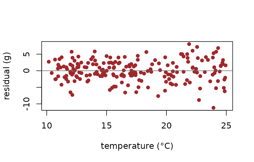

Residuals against temperature with a wedge-shaped spread

The variance is changing with temperature. A standard mixed model forces residual variance to be constant, so the inference on \beta_1 ignores that. This is called a location-scale model (also known as distributional regression or, when the variance component is what changes, heteroscedastic regression): instead of treating the residual SD as a single fixed number, we let it depend on its own predictors with its own coefficients. Climb the last rung: fit \log(\sigma_i) = \gamma_0 + \gamma_1\, T_i.

library(drmTMB)
#> 
#> Attaching package: 'drmTMB'
#> The following objects are masked from 'package:lme4':
#> 
#>     fixef, ranef
#> The following object is masked from 'package:base':
#> 
#>     beta
fit4 <- drmTMB(
  drm_formula(body_mass ~ temperature + sex + (1 | site),
              sigma     ~ temperature),
  family = gaussian(),
  data   = dat
)
sym4 <- symbolize(fit4)

equations(sym4, notation = "index")

\begin{aligned} \mathrm{body\_mass}_i \mid \mu_i,\, \sigma_i \sim \mathrm{Normal}(\mu_i,\, \sigma_i^2) \\ \mu_i = \beta_{0} + \beta_{1} \, \mathrm{temperature}_i + \beta_{2} \, [sex = \mathrm{M}] + u_{site(i)} \\ \log(\sigma_i) = \gamma_{0} + \gamma_{1} \, \mathrm{temperature}_i \\ u_{site} \sim \mathcal{N}(0,\, \sigma_{site}^2) \end{aligned}

The equation block grew by one new line — the \log(\sigma_i) = \gamma_0 + \gamma_1\, T_i row. That single additional line is the heteroscedasticity story.

Reading on the variability scale:

pi4 <- parameter_interpretation(sym4, scale = "biological")
pi4[pi4$submodel == "sigma", c("term_label", "estimate", "biological_reading")]

term_label	estimate	biological_reading
(Intercept)	0.465	Baseline level of unexplained individual variation in body_mass
temperature	0.0399	A unit change in temperature multiplies the unexplained variability of body_mass by exp(0.0399)

The slope \gamma_1 reads as “residual SD multiplies by exp(γ_1) per °C”. For our simulated data the truth was exp(0.05) ≈ 1.05, so each additional °C inflates the residual SD by about 5 %.

Three views of the same fit

For the full educator-facing surface — equation, index expansion, matrix form, with the actual numeric arrays running alongside — ask for the three-view widget:

as_html_three_views(sym4)

Skip three-views widget

What happens for each observation i – the per-individual reading.

Each observation is normally distributed around a mean that may shift with the fixed-effect predictors and a group offset, with a residual SD that may also shift with its own predictors – both location and spread are modeled.

Coefficient reading. On the response scale, \hat\beta is the additive change in the mean of the response for a one-unit increase in the predictor (identity link – no back-transformation needed).

\begin{aligned} \mathrm{body\_mass}_i \mid \mu_i,\, \sigma_i & \sim \mathrm{Normal}(\mu_i,\, \sigma_i^2) \\ \mu_i & = \beta_{0} + \beta_{1} \, \mathrm{temperature}_i + \beta_{2} \, [sex = \mathrm{M}] + u_{site(i)} \\ \log(\sigma_i) & = \gamma_{0} + \gamma_{1} \, \mathrm{temperature}_i \\ u_{site} & \sim \mathcal{N}(0,\, \sigma_{site}^2) \end{aligned}

where:

\mathrm{body\_mass}_i — response variable \mathbb{R}^{200}
\mathrm{temperature}_i — continuous predictor column of X (length 200)
\mathrm{sex}_i — factor (F [reference], M) column of X (length 200)
\mu_i — conditional mu of body_mass \mathbb{R}^{200}
\sigma_i — residual standard deviation \mathbb{R}^{200}
\beta_{0}, \beta_{1}, \beta_{2} — mu submodel coefficients \mathbb{R}^{3}
\gamma_{0}, \gamma_{1} — sigma submodel coefficients \mathbb{R}^{2}
u_{site(i)} — random intercept by site scalar; \mathbb{R}^{12} in matrix form
\sigma_{site} — between-site standard deviation scalar

Where does the variation live? Where the variation lives – each row is one variance component (shown as a share of the total when a single total variance is defined).

site: variance = 1.28

ICC: ICC not available on this scale yet. (the residual SD varies across observations (a location-scale model), so there is no single within-group variance to form the ICC.)

Point estimates only; uncertainty not shown.

The same matrix equation, with your actual numbers stacked inside the brackets – what the computer multiplies. Showing first 5 and last 2 rows of n = 200.

Each observation is normally distributed around a mean that may shift with the fixed-effect predictors and a group offset, with a residual SD that may also shift with its own predictors – both location and spread are modeled.

For observation i = 1 of your data:

\begin{aligned} \mathrm{body\_mass}_{1} &= \hat\beta_{0} + \hat\beta_{1}\,\mathrm{temperature}_{1} + \hat\beta_{2}\,\mathrm{sexM}_{1} + \hat{u}_{\mathrm{site},\,\mathrm{S01}} + \hat\varepsilon_{1} &\quad(\text{response equation, one row of the model}) \\ \hat\mu_{1} &= 32.1 + 0.3 \times 23.9 + 0.757 \times 0 + (-1.33) \approx 37.9 &\quad(\text{predicted mean} = \text{linear predictor}) \\ \mathrm{body\_mass}_{1} &= \underbrace{37.9}_{\textstyle\,\hat\mu_{1}\,\text{(predicted)}\,} \;+\; \underbrace{(-1.06)}_{\textstyle\,\hat\varepsilon_{1}\,\text{(residual)}\,} &\quad(\text{observed} = \text{predicted mean} + \text{residual}) \end{aligned}

Stacking the same response equation for all n = 200 observations:

\underbrace{\begin{bmatrix} 36.8 \\ 32.9 \\ 37.7 \\ 40.2 \\ 36.1 \\ \vdots \\ 38 \\ 38.3 \end{bmatrix}}_{\textstyle\,\mathbf{body\_mass}_{\,200 \times 1}\;\text{(observed)}\,} \;=\; \underbrace{\begin{bmatrix} 1 & 23.9 & 0 \\ 1 & 17.7 & 0 \\ 1 & 13.9 & 1 \\ 1 & 10.7 & 0 \\ 1 & 16.3 & 0 \\ \vdots & \vdots & \vdots \\ 1 & 19.9 & 1 \\ 1 & 12.1 & 1 \end{bmatrix}}_{\textstyle\,\mathbf{X}_{\,200 \times 3}\,}\, \underbrace{\begin{bmatrix} 32.1 \\ 0.3 \\ 0.757 \end{bmatrix}}_{\textstyle\,\hat{\boldsymbol{\beta}}_{\,3 \times 1}\;\text{(estimated)}\,} \;+\; \underbrace{\begin{bmatrix} 1 & 0 & 0 & 0 & 0 & \cdots & 0 & 0 \\ 0 & 1 & 0 & 0 & 0 & \cdots & 0 & 0 \\ 0 & 0 & 1 & 0 & 0 & \cdots & 0 & 0 \\ 0 & 0 & 0 & 1 & 0 & \cdots & 0 & 0 \\ 0 & 0 & 0 & 0 & 1 & \cdots & 0 & 0 \\ \vdots & \vdots & \vdots & \vdots & \vdots & \ddots & \vdots & \vdots \\ 0 & 0 & 0 & 0 & 0 & \cdots & 1 & 0 \\ 0 & 0 & 0 & 0 & 0 & \cdots & 0 & 1 \end{bmatrix}}_{\textstyle\,\mathbf{Z}_{\text{site},\,\,200 \times 12}\,}\, \underbrace{\begin{bmatrix} -1.33 \\ 0.266 \\ -1.38 \\ 1.48 \\ 0.519 \\ \vdots \\ -0.247 \\ 0.281 \end{bmatrix}}_{\textstyle\,\hat{\mathbf{u}}_{\text{site},\,12 \times 1}\;\text{(BLUP)}\,} \;+\; \underbrace{\begin{bmatrix} -1.06 \\ -4.76 \\ 2.06 \\ 3.42 \\ -1.4 \\ \vdots \\ -0.568 \\ 1.54 \end{bmatrix}}_{\textstyle\,\hat{\boldsymbol{\varepsilon}}_{\,200 \times 1}\;\text{(residual)}\,}

Left: observed vector \mathbf{body\_mass}. Middle: the prediction \mathbf{X}\hat{\boldsymbol{\beta}} + \mathbf{Z}\hat{\mathbf{u}} = \hat{\boldsymbol{\mu}}. Right: the residual vector \hat{\boldsymbol{\varepsilon}} = \mathbf{body\_mass} - \hat{\boldsymbol{\mu}}. Every row of this matrix equation is one of the response-equation rows from the worked row above.

Partial pooling. The random-effect estimates shown here (the BLUPs) are partially pooled: each group’s estimate is shrunk toward zero by an amount that grows when the group has little data and shrinks when the between-group variance is large. Groups with the least data are pulled hardest toward the overall mean.

And the \sigma submodel (no observed counterpart – \sigma’s job is to describe the spread of \hat{\boldsymbol{\varepsilon}}). For the same observation i = 1:

\begin{aligned} \log\hat\sigma_{1} &= \hat\gamma_{0} + \hat\gamma_{1}\,\mathrm{temperature}_{1} &\quad(\text{sigma submodel for observation 1, log link}) \\ \log\hat\sigma_{1} &= 0.465 + 0.0399 \times 23.9 = 1.42 &\quad(\text{with your numbers}) \\ \hat\sigma_{1} &= \exp(1.42) \approx 4.12 &\quad(\text{predicted residual SD for observation 1}) \end{aligned}

Stacking the same log-link equation for all n = 200 observations:

\log\!\underbrace{\begin{bmatrix} 4.12 \\ 3.22 \\ 2.77 \\ 2.44 \\ 3.04 \\ \vdots \\ 3.53 \\ 2.58 \end{bmatrix}}_{\textstyle\,\boldsymbol{\sigma}_{\,200 \times 1}\,} \;=\; \underbrace{\begin{bmatrix} 1 & 23.9 \\ 1 & 17.7 \\ 1 & 13.9 \\ 1 & 10.7 \\ 1 & 16.3 \\ \vdots & \vdots \\ 1 & 19.9 \\ 1 & 12.1 \end{bmatrix}}_{\textstyle\,\mathbf{X}_{\sigma,\,200 \times 2}\,}\, \underbrace{\begin{bmatrix} 0.465 \\ 0.0399 \end{bmatrix}}_{\textstyle\,\boldsymbol{\gamma}_{\,2 \times 1}\,}

(The widget renders live in this page. In an R session, cat(as_html_three_views(sym)) inside a results = "asis" chunk will render the same widget into a knitted document.)

What just happened: a recap

Rung	Equation	New rows in symbolize output
1: `lm`	y_i \sim \mathcal{N}(\mu_i,\, \sigma^2); \mu_i = \beta_0 + \beta_1 T_i	distribution + linear predictor
2: `lm + sex`	\mu_i = \beta_0 + \beta_1 T_i + \beta_2 [\mathit{sex} = M]	factor contrast row in `symbol_table` / interp
3: `lmer + (1\|site)`	\mu_i = \beta_0 + \beta_1 T_i + \beta_2 [\mathit{sex} = M] + u_{site(i)}; u_{site} \sim \mathcal{N}(0,\, \sigma^2_{site})	random-effect symbol + `variance_components` rows
4: `drmTMB` location-scale	as Rung 3, plus \log(\sigma_i) = \gamma_0 + \gamma_1 T_i	`sigma` submodel + heteroscedasticity reading

Three observations:

The same symbolize() call works on every fit. No class-specific accessors. The four fits cover three different packages (stats, lme4, drmTMB) and the user-facing surface is identical.
The equation block grows exactly where the model grows. Each rung adds one concept; the LaTeX line count tells you which.
The symbolic surface is incrementally readable. A student who just learned lm can read Rung 1; a student who just learned random effects can read Rung 3 and see what Rung 4 adds on top.

The same approach scales to every model class symbolizer covers — glmmTMB, brms, MCMCglmm, sdmTMB, metafor, mgcv. The educator-facing surface stays one verb deep.

Where to next

For factor / interaction pedagogy in depth, see vignette("symbolizer-factors").
For a tour of distributional families (Student-t, Gamma, beta, binomial, …), see vignette("symbolizer-families").
For meta-analysis with metafor and drmTMB location-scale (plus glmmTMB’s propto() as the related phylogenetic / structured-covariance pattern, not strict meta-analysis), see vignette("symbolizer-meta-analysis").
For the full capability matrix and what’s planned next, see vignette("symbolizer-roadmap").